Introduction
我们平时在做科研的时候,经常会遇到需要整理文献信息的情况。比如,我们需要查找某个领域的最新论文,或者是了解一个作者的发文情况等等。
一般情况下,我们会通过搜索引擎来查找相关的文献,然后逐一查看。但手动的话一般很难快速整理成表,所以我在这里简单介绍几个R包,可以帮助我们快速整理文献信息:
scholar
Google Scholar 可能是了解一位作者最好的途径了(如果他有账号的话,因为这里的list一般比较全。但由于没有ORCID一类的标识符,也可能出现不是该作者的文章)。scholar包提供从 Google Scholar 中提取引文数据的功能。还提供了方便的函数来比较多个学者并预测未来的 H 指数值。
1
2
3
4
5
6
|
# from CRAN
install.packages("scholar")

# from GitHub
if(!requireNamespace('remotes')) install.packages("remotes")
remotes::install_github('YuLab-SMU/scholar')
|
注意使用这个包需要我们本来就能上Google Scholar(代理一下),然后记得在R环境里也设置一下:
1
2
3
4
5
|
# install.packages("r.proxy")

r.proxy::proxy() #打开代理

# r.proxy::noproxy() #不用的话可以关掉
|
获取作者的profile
 1
 2
 3
 4
 5
 6
 7
 8
 9
10
11
12
13
14
15
16
17
18
19
20
21
22
23
24
25
|
library(scholar)
## Define the id for Richard Feynman,这个id可以在Google Scholar中找到,看网址中的user=XXXXXXXXX
id <- 'B7vSqZsAAAAJ'

## Get his profile
l <- get_profile(id)

print(l[2:7])
## $name
## [1] "Richard Feynman"
##
## $affiliation
## [1] "California Institute of Technology"
##
## $total_cites
## [1] 127275
##
## $h_index
## [1] 62
##
## $i10_index
## [1] 100
##
## $fields
## [1] "quantum mechanics"       "quantum electrodynamics"
|
获取作者的文章列表
1
2
3
|
pubdf=get_publications(id)
nrow(pubdf)
## [1] 157
|
注意这里的文章信息并不多,只有标题、作者列表、期刊、发表年、引用量等。而且,作者列表里如果人名太多太长,就会出现"…“的省略😂,我们可以进一步处理:
 1
 2
 3
 4
 5
 6
 7
 8
 9
10
11
12
13
14
15
|
# 比如pubdf$author[33]
# "RP Feynman, RB Leighton, M Sands, CA Heras, R Gómez, E Oelker, ..."

for (i in 1:nrow(pubdf)){
    if (grepl("...", pubdf$author[i],fixed = TRUE)) {
        pubdf$author[i] <- get_complete_authors(id,pubdf$pubid[i])
    }
}

# 处理好之后:
# "RP Feynman, RB Leighton, M Sands, CA Heras, R Gómez, E Oelker, H Espinosa"

# 获取作者排名(根据姓查询的,比如这里就是用Feynman,有重名的话保留靠前的排名):
author_pos=scholar::author_position(pubdf$author,l$name)
pubdf=cbind(pubdf,author_pos)
|
这里的Position_Normalized基本可以确定0是第一作者,1是最后一个通讯作者了,但是共一共通讯需要自己去手动看看。
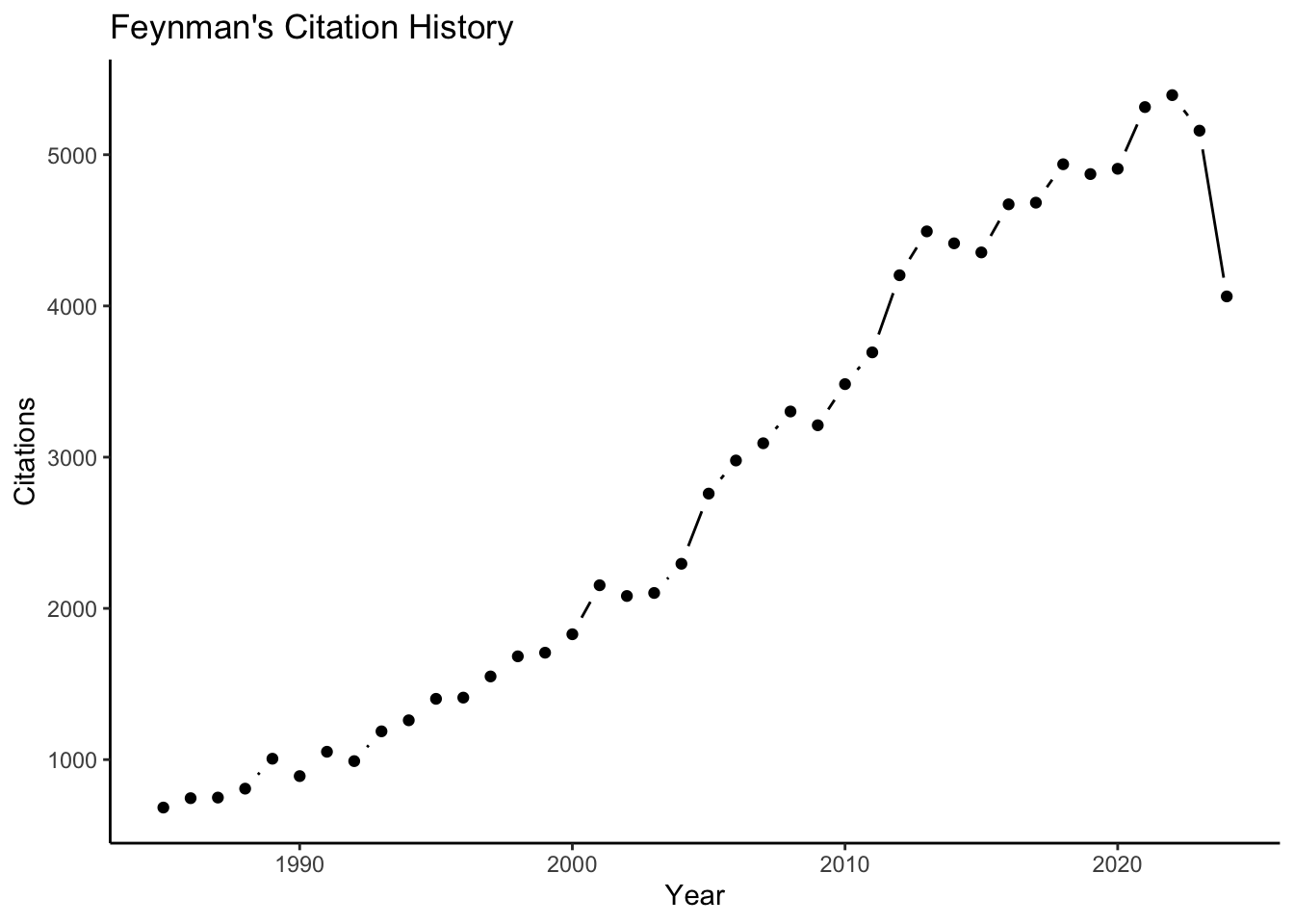
引用次数可视化
1
2
3
4
5
6
7
8
9
|
#作者年份被引信息
scholar::get_citation_history(id)->citation_history
#某一篇文章年份被引信息
scholar::get_article_cite_history(id,pubdf$pubid[1])->article_cite_history

ggplot(citation_history,aes(x=year,y=cites)) +
    ggh4x::geom_pointpath()+
    labs(title="Feynman's Citation History",x="Year",y="Citations")+
    theme_classic()
|
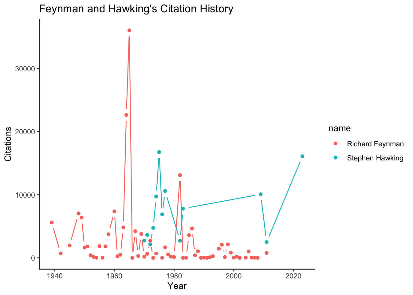
作者比较
1
2
3
4
5
6
7
|
#比较Feynman和Hawking的文章引用
compare_scholars(c('B7vSqZsAAAAJ', 'qj74uXkAAAAJ'))->compare_result

ggplot(compare_result,aes(x=year,y=cites,color=name)) +
    ggh4x::geom_pointpath()+
    labs(title="Feynman and Hawking's Citation History",x="Year",y="Citations")+
    theme_classic()
|
1
2
3
4
5
6
7
|
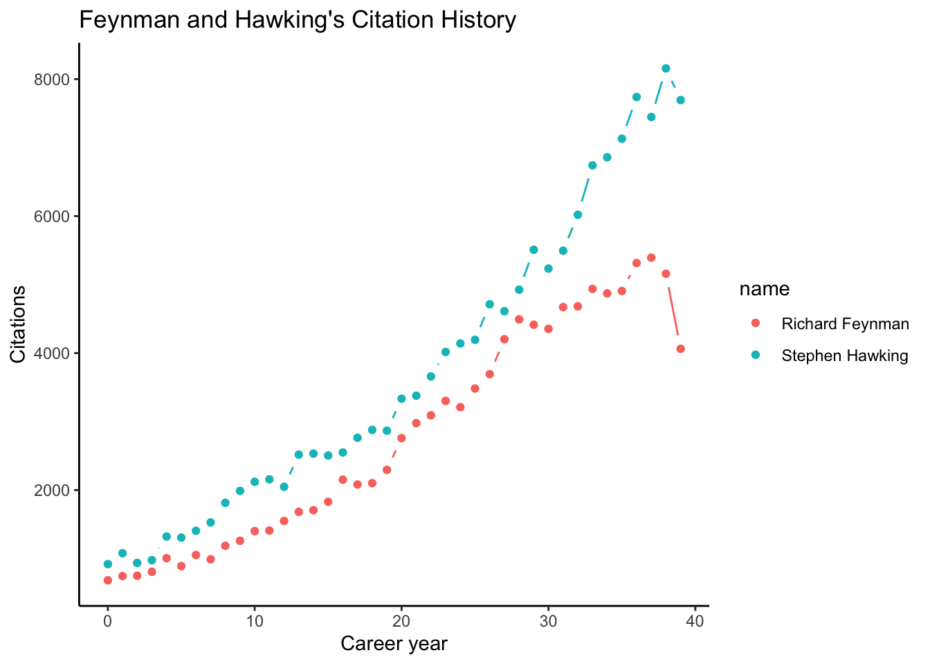
#用职业生涯比较累计量
compare_scholar_careers(c('B7vSqZsAAAAJ', 'qj74uXkAAAAJ'))->compare_career_result
ggplot(compare_career_result,aes(x=career_year,y=cites,color=name)) +
    ggh4x::geom_pointpath()+
    labs(title="Feynman and Hawking's Citation History",x="Career year",y="Citations")+
    theme_classic()
|
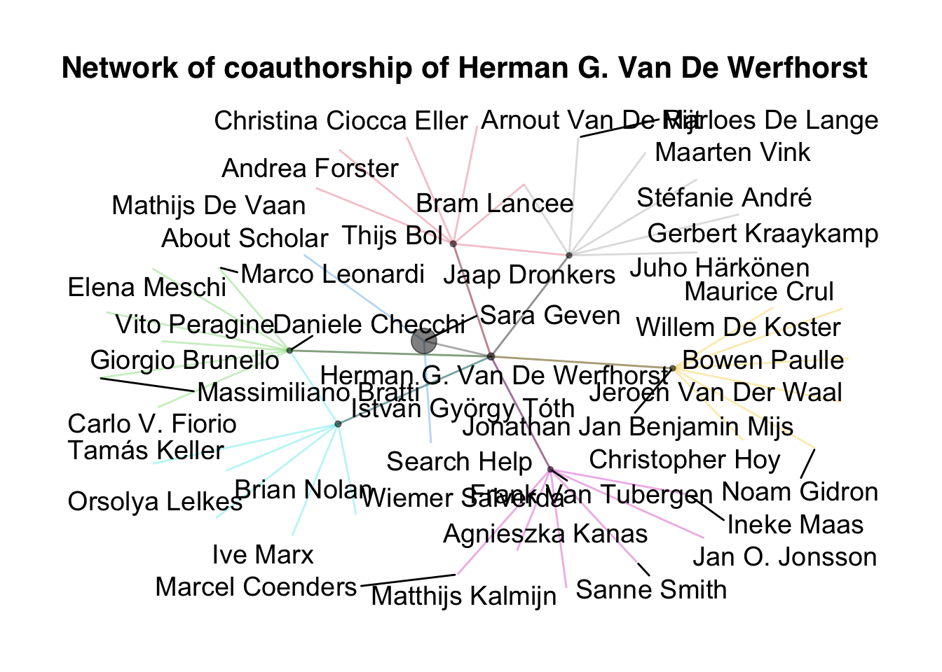
作者的co-author网络
1
2
|
coauthor_network <- get_coauthors("amYIKXQAAAAJ&hl", n_coauthors = 7)
plot_coauthors(coauthor_network)
|
预测未来的h指数值
1
2
3
|
## Predict h-index of original method author, Daniel Acuna
id <- 'GAi23ssAAAAJ'
predict_h_index(id)
|
rcrossref
DOI (Digital Object Identifier) 是一种唯一的、永久的数字标识符,用于标记学术文章、图书、数据集等数字内容,确保即使资源位置变化,用户仍能访问。DOI由国际DOI基金会管理,广泛用于出版和学术界。
Crossref 是一家非营利组织,负责为出版物分配和管理DOI。它通过与出版商合作,使学术资源能够通过DOI轻松发现和引用。Crossref 提供的服务帮助提升了学术成果的可追溯性和引用率。
rcrossref 是一款 R 语言包,其核心功能是与 CrossRef 平台进行交互,实现对全球数千万条文献记录的快速查询和处理。通过该包,用户可以方便地获取论文的DOI(数字对象唯一标识符)、作者信息、出版年份等详细元数据,甚至进行文本和数据挖掘服务。
1
2
3
4
|
# from CRAN
install.packages("rcrossref")
# from GitHub
remotes::install_github("ropensci/rcrossref")
|
通过DOI获取文章信息
如果我们有文章的DOI,可以通过rcrossref包获取文章的元数据,这是最方便的。
1
2
3
4
5
6
|
library(rcrossref)
cr_works(dois='10.1063/1.3593378')->doi_res
#批量查询也是可以的

cr_works(dois=c('10.1007/12080.1874-1746','10.1007/10452.1573-5125',
   '10.1111/(issn)1442-9993'),.progress = "text")# 加上进度条
|
doi_res$data里面提供了非常详细的信息,包括作者列表、标题、出版年份、参考文献等,可以进一步整理表格。
通过其他信息查询文章
官网提供了https://docs.ropensci.org/rcrossref/articles/crossref_filters.html,可以根据作者、关键词、出版时间等信息进行筛选。
 1
 2
 3
 4
 5
 6
 7
 8
 9
10
|
library(rcrossref)
# 通过作者ORCID查询文章,但不是很准确,会少很多
cr_works(filter = list(orcid="0000-0002-9449-7606"))->orcid_res

# 通过期刊+标题查询文章(比如我们之前谷歌学术的结果表格只有期刊+标题,一般没有DOI)
res <- cr_works(query = "Interaction with the absorber as the mechanism of radiation",
                flq = c(`query.container-title` = 'Reviews of Modern Physics'))
# 这个可能会搜到很多结果,一般第一条是比较准确的,可以手动check一下:
nrow(res$data)
## [1] 20
|
举个例子,我们需要将上面找到的谷歌学术列表中的文章表格添加DOI信息,可以用下列代码:
 1
 2
 3
 4
 5
 6
 7
 8
 9
10
11
12
13
14
15
16
17
18
|
library(rcrossref)
pubdf2=get_publications(id)
pubdf2$DOI=NA

for (i in seq_len(nrow(pubdf2))){
    results <- cr_works(query = pubdf2$title[i], filter = c(type = "journal-article"))
    if(stringr::str_equal(pubdf2$title[i],results$data$title[1],ignore_case = T)){
        # 如果第一篇文章标题和搜索结果标题完全一致,则添加DOI
        pubdf2$DOI[i]=results$data$doi[1]
    } else{
        # 如果第一篇文章标题和搜索结果标题不完全一致,则需要手动选择
        cat(pubdf2$title[i],"\n\n",results$data$title[1])
        flag <- readline("yes/no(y/n)?")
        if (tolower(flag) %in% c("yes", "y")) {
             pubdf2$DOI[i]=results$data$doi[1]
        }
    }
}
|
PubMed相关R包
PubMed数据库是一个流行的数据库(但我用的比较少😂,基本上直接谷歌学术),有很多包可以用来查询PubMed数据库并挖掘,比如RISmed,pumed.mineR,easyPubMed等等。
RISmed
这是一套从国家生物技术信息中心(NCBI)数据库(包括PubMed)中提取书目内容的工具。RISmed是RIS(用于研究信息系统,书目数据的通用标签格式)和PubMed的组合。
 1
 2
 3
 4
 5
 6
 7
 8
 9
10
11
12
|
library(RISmed)

# 限定检索主题
search_topic<-"indoor air microbiome"
search_query<-EUtilsSummary(search_topic,db="pubmed",type="esearch",mindate=2022,maxdate=2024)
summary(search_query)

# 获取摘要信息,经常有网络问题😂不如去网站检索再导出
records<- EUtilsGet(search_query@PMID,type="efetch",db="pubmed")

# 获取作者信息
authors <- Author(records)
|
easyPubMed
EasyPubMed是Entrez编程实用程序的开源R接口,旨在允许在R环境中对PubMed进行程序化访问。该软件包适用于下载大量记录,并包含一系列功能来执行Entrez/PubMed查询响应的基本处理。该库支持XML或TXT(“ MEDLINE”)格式。
 1
 2
 3
 4
 5
 6
 7
 8
 9
10
11
12
13
14
15
16
17
18
19
20
21
22
23
24
25
|
library(easyPubMed)

# 可以直接输入文章标题查找
fullti <- get_pubmed_ids_by_fulltitle(
    fulltitle = "Identification of hub genes and outcome in colon cancer based on bioinformatics analysis",
    field = "[Title]")

# PMID
fullti$IdList$Id
## [1] "30643458"

# 转为DOI
rcrossref::id_converter(fullti$IdList$Id)
## $status
## [1] "ok"
##
## $responseDate
## [1] "2024-10-14 02:56:51"
##
## $request
## [1] "tool=rcrossref;email=myrmecocystus%40gmail.com;ids=30643458;format=json"
##
## $records
##        pmcid     pmid                  doi           versions
## 1 PMC6312054 30643458 10.2147/CMAR.S173240 PMC6312054.1, true
|
bibliometrix
BiblioMetrix软件包提供了一组用于文献计量学和科学计量学方面的定量研究的工具。
文献计量学本身是科学,定量分析的主要工具。本质上,书目计量学是定量分析和统计数据的应用,例如期刊文章及其随附的引文数。现在,几乎所有科学领域都使用了对出版和引文数据的定量评估,以评估成长,成熟度,主要作者,概念图和智力图,科学界的趋势。
BIBLIOMERTIC还用于研究绩效评估,尤其是在大学和政府实验室,以及决策者,研究总监和管理人员,信息专家和图书馆员以及学者本身。
BiblioMetrix在分析的三个关键阶段支持学者:
- 数据导入和转换为R格式;
- 出版数据集的文献计量分析;
- 构建和绘制矩阵,用于共同引用,耦合,协作和共同词分析。矩阵是用于执行网络分析,多个对应分析和任何其他数据减少技术的输入数据。
这个包的使用教程很多,比如参考https://blog.csdn.net/weixin_42487488/article/details/116379324。而且它提供一个shiny界面,不需要很多代码知识也可以方便使用。
数据获取
一般使用自己检索或整理得到的bib文件,比如直接从web of science检索,export为BibTex;或者自己想去看的某个作者的文章列表。
 1
 2
 3
 4
 5
 6
 7
 8
 9
10
11
12
13
|
library(bibliometrix)

file <- c("https://www.bibliometrix.org/datasets/management1.txt",
          "https://www.bibliometrix.org/datasets/management2.txt")

M <- convert2df(file = file, dbsource = "wos", format = "plaintext")
##
## Converting your wos collection into a bibliographic dataframe
##
## Done!
##
##
## Generating affiliation field tag AU_UN from C1:  Done!
|
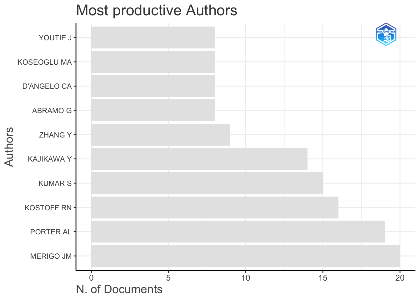
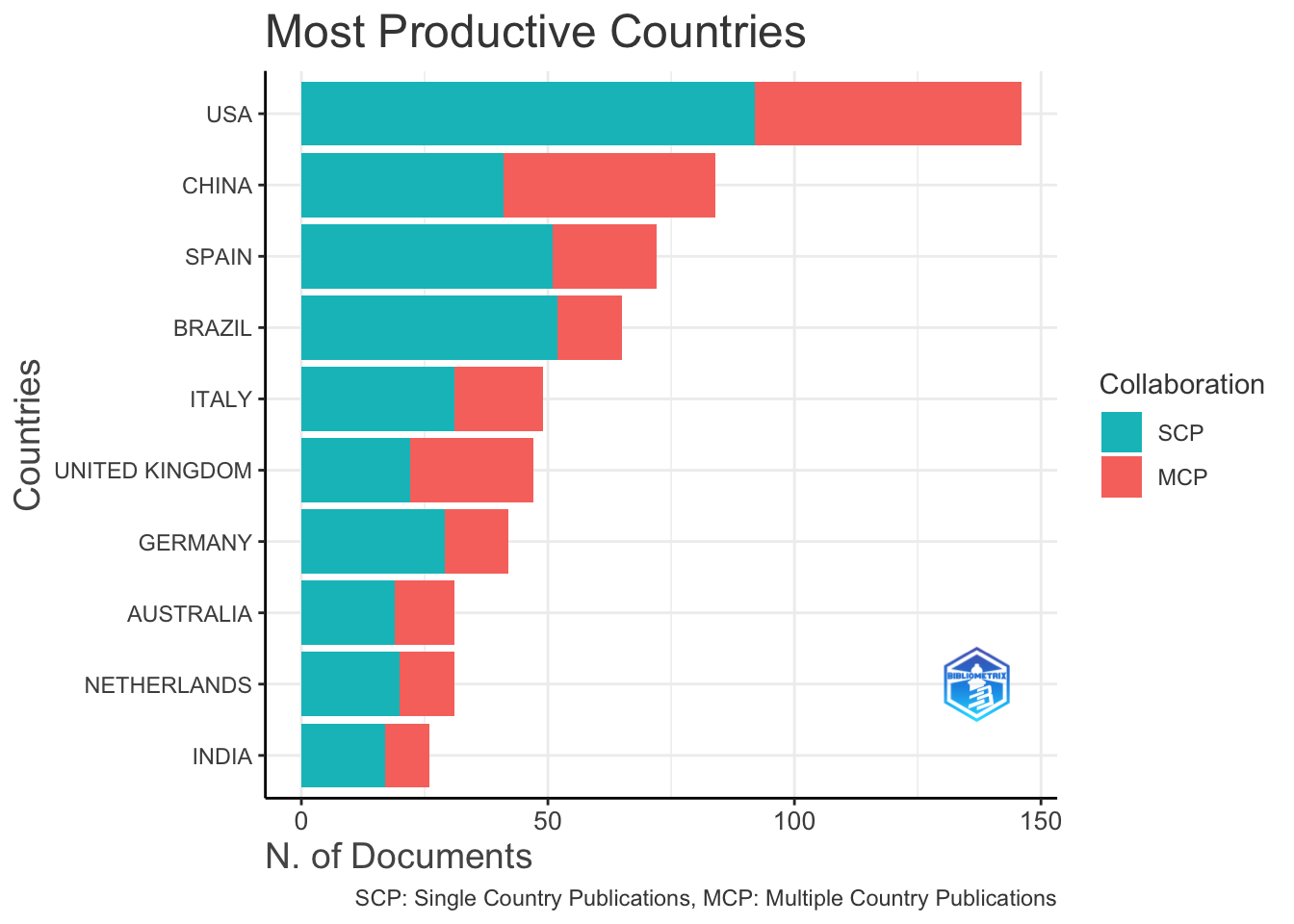
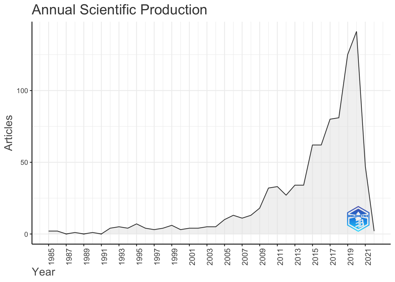
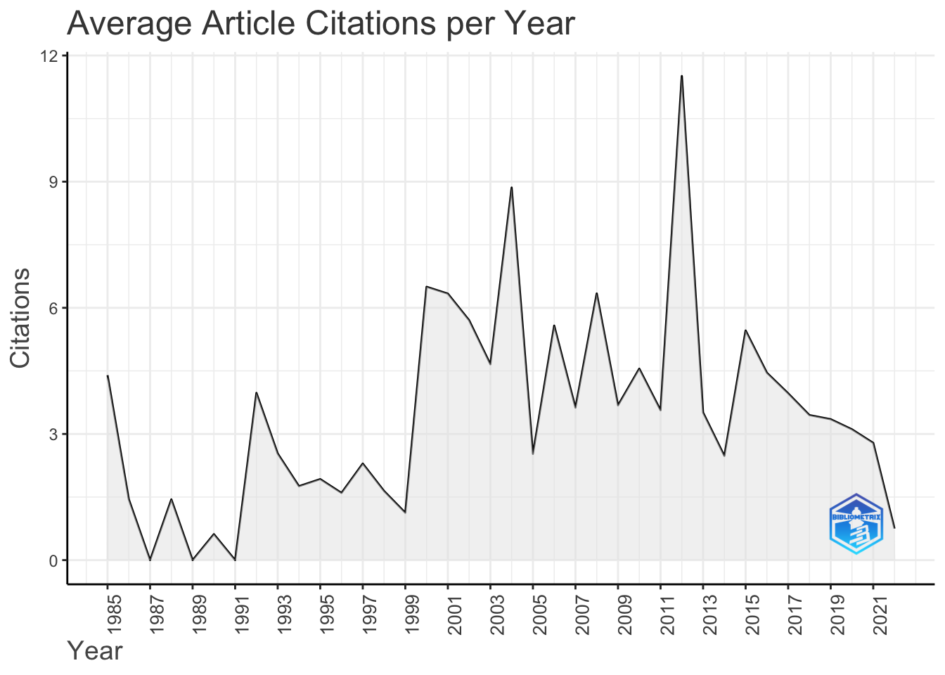
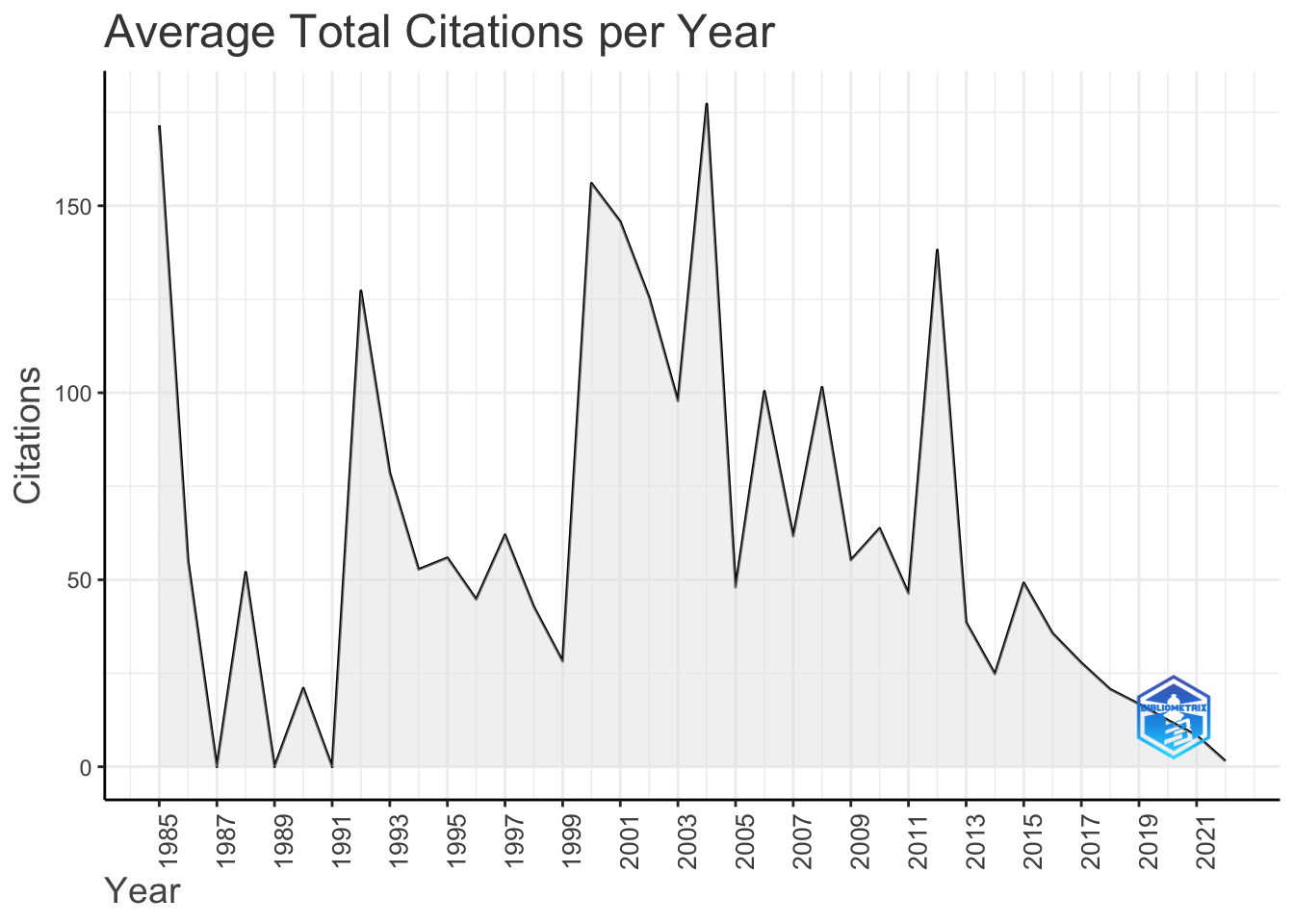
基本信息
1
2
3
|
results <- biblioAnalysis(M, sep = ";")

plot(x = results, k = 10, pause = FALSE)
|
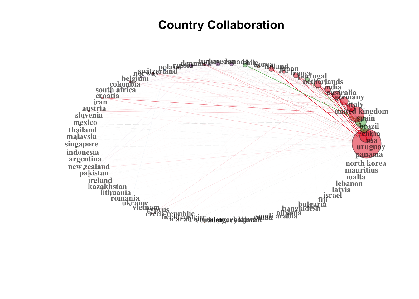
可视化文献网络
展示国家科学合作:
1
2
3
4
5
6
7
8
|
# Create a country collaboration network

M <- metaTagExtraction(M, Field = "AU_CO", sep = ";")
NetMatrix <- biblioNetwork(M, analysis = "collaboration", network = "countries", sep = ";")

# Plot the network
net=networkPlot(NetMatrix, n = dim(NetMatrix)[1], Title = "Country Collaboration",
                type = "circle", size=TRUE, remove.multiple=FALSE,labelsize=0.8)
|
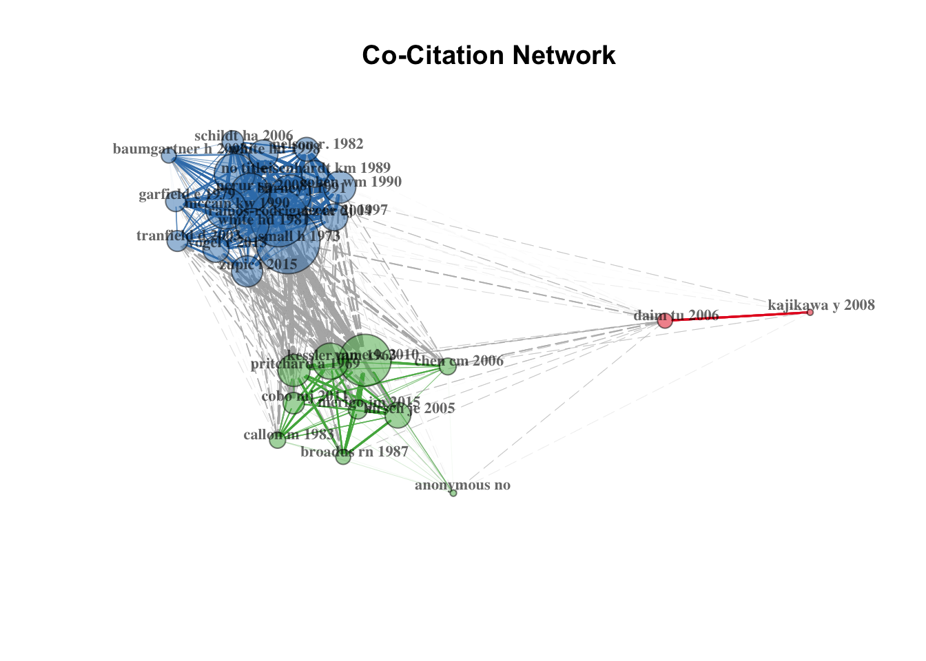
共同引用分析:
1
2
3
4
5
6
7
|
# Create a co-citation network

NetMatrix <- biblioNetwork(M, analysis = "co-citation", network = "references", n=30, sep = ";")

# Plot the network
net=networkPlot(NetMatrix, Title = "Co-Citation Network", type = "fruchterman",
                size=T, remove.multiple=FALSE, labelsize=0.7,edgesize = 5)
|
 关键词网络:
1
2
3
4
5
6
7
8
|
# Create keyword co-occurrences network

NetMatrix <- biblioNetwork(M, analysis = "co-occurrences", network = "keywords", sep = ";")

# Plot the network
net=networkPlot(NetMatrix, normalize="association", weighted=T, n = 30,
                Title = "Keyword Co-occurrences", type = "fruchterman",
                size=T,edgesize = 5,labelsize=0.7)
|

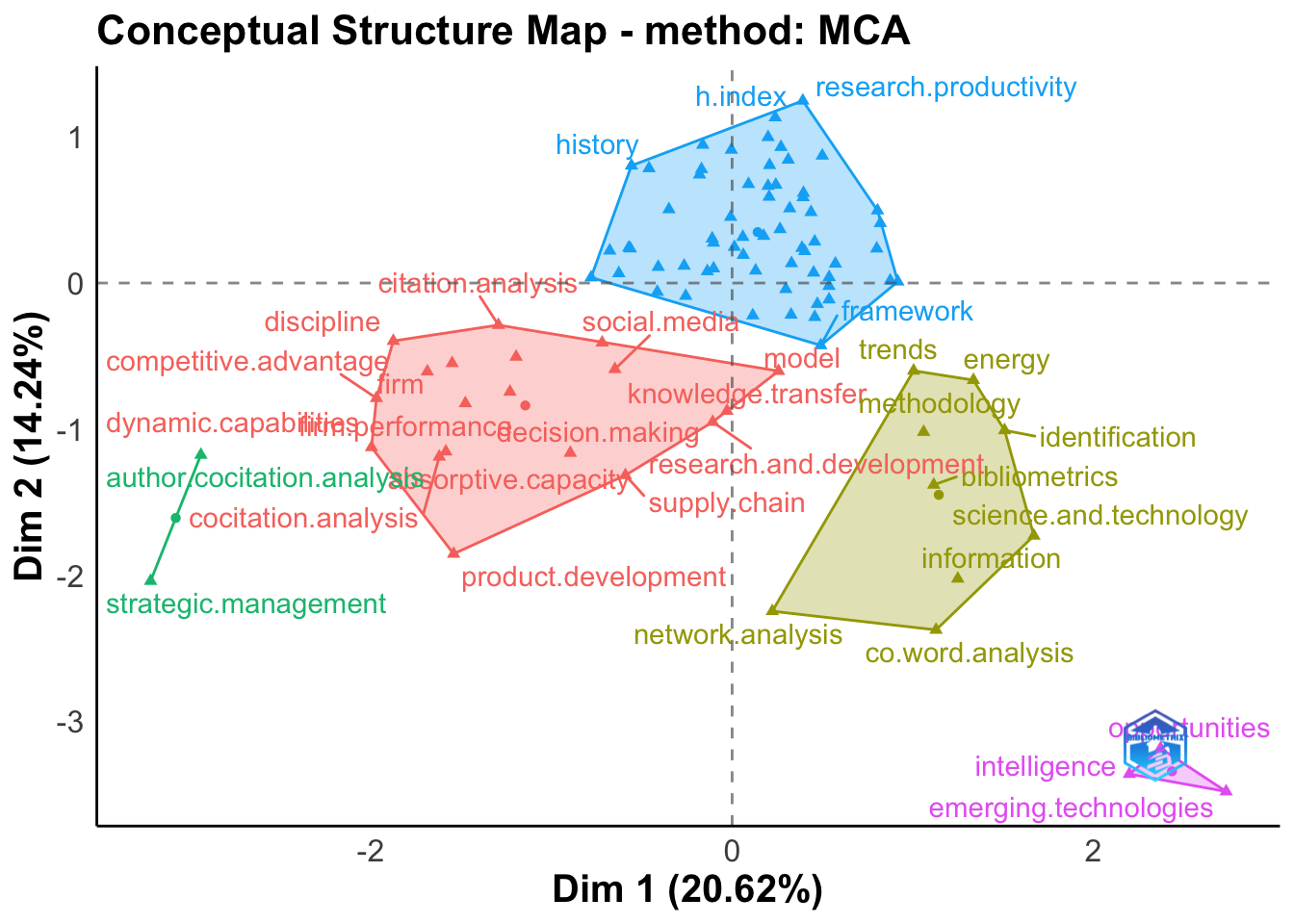
Co-Word分析
共词分析的目的是使用书目集合中的词共现来映射框架的概念结构。
可以通过降维技术(例如多维标度(MDS)、对应分析(CA)或多对应分析(MCA))来执行分析。
这里展示了一个使用函数 ConceptualStructure 的示例,该函数执行 CA 或 MCA 来绘制字段的概念结构,并使用 K 均值聚类来识别表达共同概念的文档簇。结果绘制在二维图上。
1
2
3
4
5
|
# Conceptual Structure using keywords (method="CA")

CS <- conceptualStructure(M,field="ID", method="MCA", minDegree=10, clust=5,
                          stemming=FALSE, labelsize=15, documents=20, graph=FALSE)
plot(CS$graph_terms)
|
其他需求
添加期刊影响因子
目前没有特别好的R包或函数来获取期刊的影响因子,之前scholar包 get_impactfactor函数也无法使用了。最好的方法还是自己去下载一下当年的JCR影响因子表格(很多公众号都可以获取),然后自己用R整合一下。我之前也也简单整理了一个IF大于2.4的部分期刊的表,下载链接:https://asa12138.github.io/FileList/JCR_IF_2024_bigger_than_2.4.csv。
1
2
3
4
5
6
7
8
9
|
#获取IF
readr::read_csv("~/Documents/Others/JCRs/JCR_IF_2024_bigger_than_2.4.csv")->jcr_df
pubdf2$IF=NA
for (i in seq_len(nrow(pubdf2))){
    tmp=which(stringr::str_equal(pubdf2$journal[i],jcr_df$`Journal name`,ignore_case = T))
    if (length(tmp)>0) {
         pubdf2$IF[i]=jcr_df[tmp,3]%>%unlist()
    }
}
|