之前已经介绍了网络计算,构建以及各种注释了。本文将详细介绍MetaNet中的各种可视化方法,从基础绘图到高级布局技巧。
- 软件主页:https://github.com/Asa12138/MetaNet 大家可以帮忙在github上点点star⭐️,谢谢🙏
- 详细英文版教程:https://bookdown.org/Asa12138/metanet_book/
可以从 CRAN 安装稳定版:install.packages("MetaNet")
最新的开发版本可以在 https://github.com/Asa12138/MetaNet 中找到:
|
|
依赖包 pcutils和igraph(需提前安装),推荐配合 dplyr 进行数据操作。
|
|
绘图设置
在构建网络时,MetaNet已经设置了一些与可视化相关的内部属性。我们可以使用c_net_set()函数自定义这些属性以满足研究需求。
如果需要更灵活地自定义网络图,可以使用c_net_plot()函数,它包含许多灵活的绘图参数:


示例代码,尝试各种设置看看:
|
|
使用params_list
params_list是c_net_plot()中的一个特殊参数,它是一个包含参数的列表,可以方便地用于绘制一系列具有相同属性的网络图:
|
|
|
|
网络布局
布局是网络可视化的重要组成部分,一个好的布局可以清晰地呈现信息。
在MetaNet中,我们使用coors对象来存储布局的坐标。coors是一个具有"name", “X”, “Y"三列的dataframe。
基础布局
使用c_net_layout()获取特定布局方法的坐标:
|
|
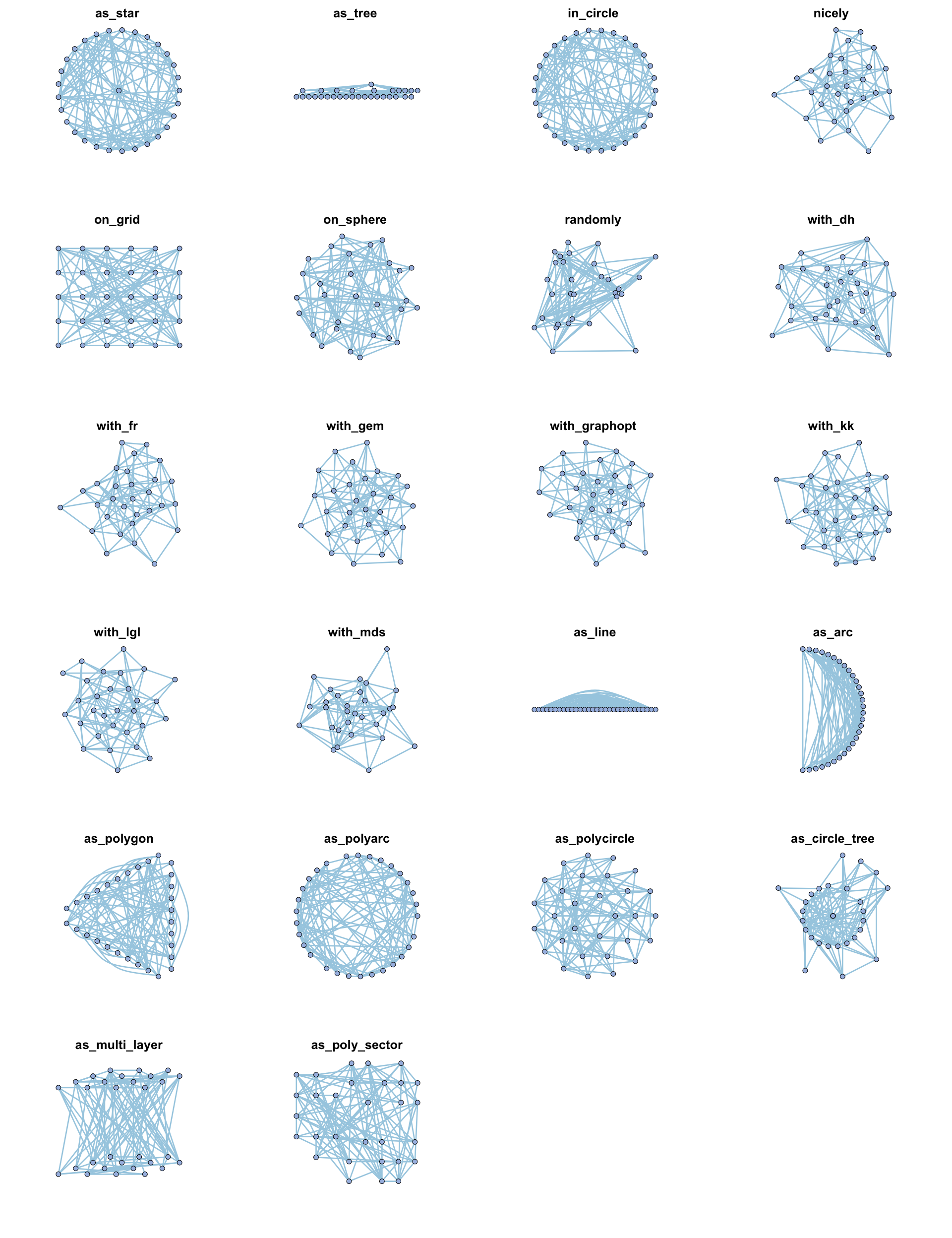
可用的基础布局方法包括:
- igraph布局:
in_circle(),nicely(),on_grid(),on_sphere(),randomly(),with_dh(),with_fr(),with_gem(),with_graphopt(),with_kk(),with_lgl(),with_mds() - metanet新布局方法:
as_line(),as_arc(),as_polygon(),as_polyarc(),as_polycircle(),as_circle_tree(),as_multi_layer(),as_poly_sector() - ggraph布局:“auto”, “backbone”, “centrality”, “circlepack”, “dendrogram”, “eigen”, “focus”, “hive”, “igraph”, “linear”, “manual”, “matrix”, “partition”, “pmds”, “stress”, “treemap”, “unrooted”
示例代码展示不同布局效果:
|
|
 对于每种方法,可以在其中额外添加一些参数:
|
|
as_polygon()很有趣,它可以绘制多边形形状的网络,您可以更改多边形的边数:
变换布局
使用transform_comors可以转换布局,包括缩放,X/Y比,旋转角度,镜像,伪3D效果等:
|
|
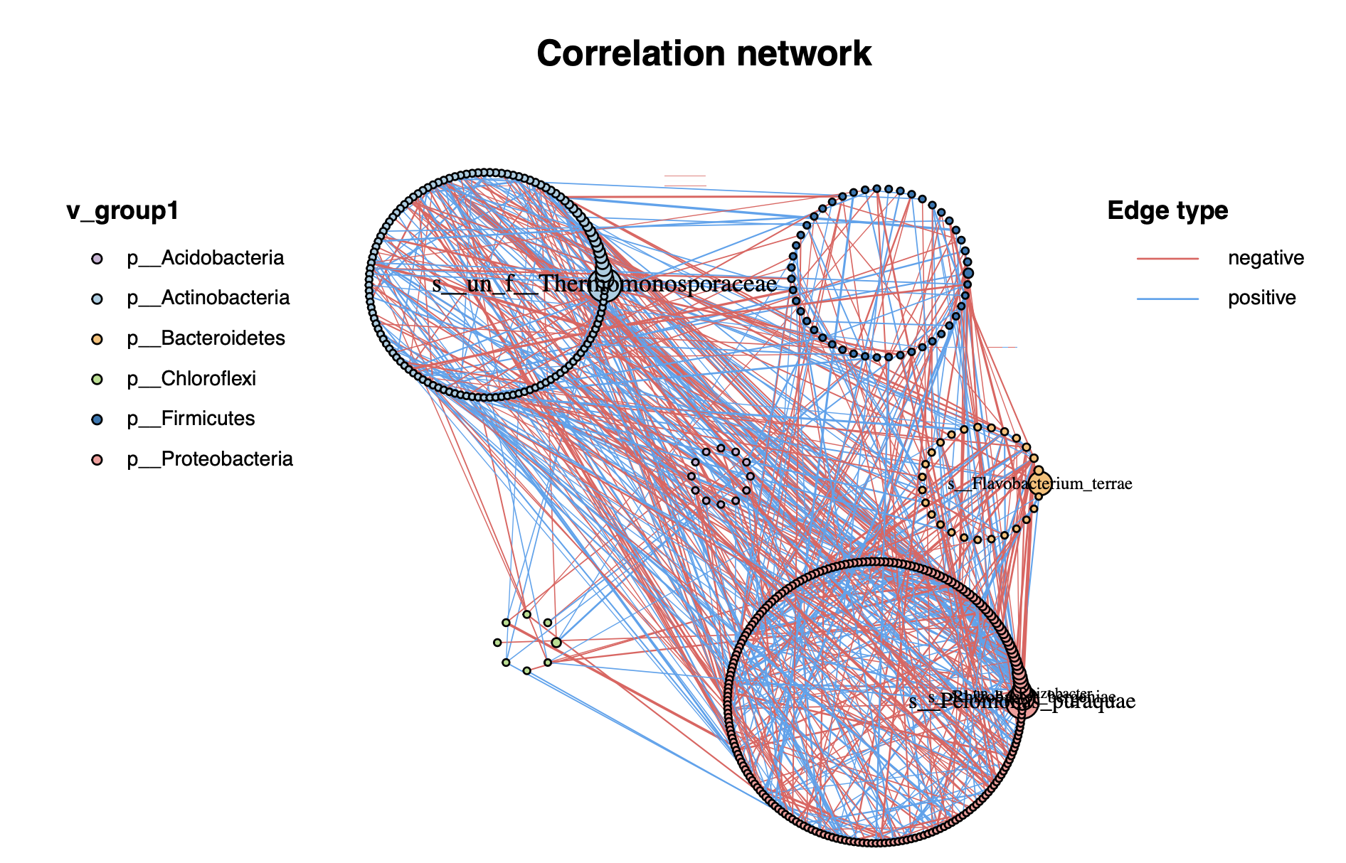
分组布局
除c_net_layout()外,我们还为具有分组变量的网络提供了一种高级布局方法:g_layout()。
使用g_layout()可以轻松控制每个组的位置及其内部布局。g_layout()返回的也是coors对象,这意味着我们可以继续用g_layout()组合,实现疯狂套娃,高度自定义的布局!
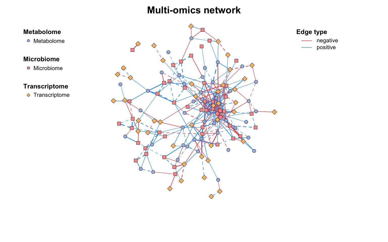
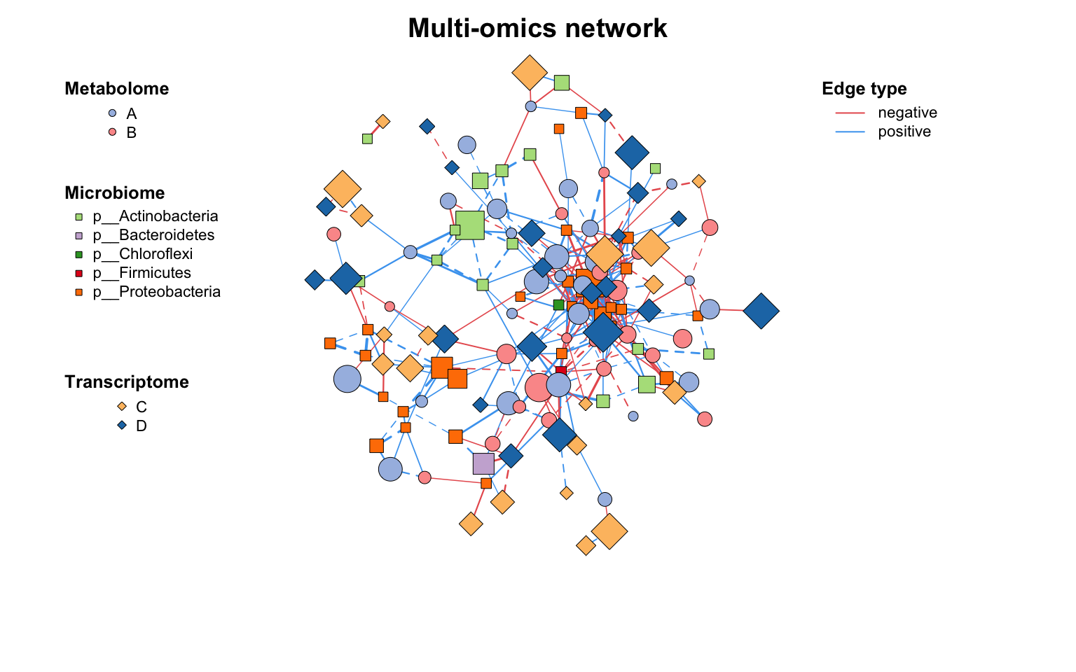
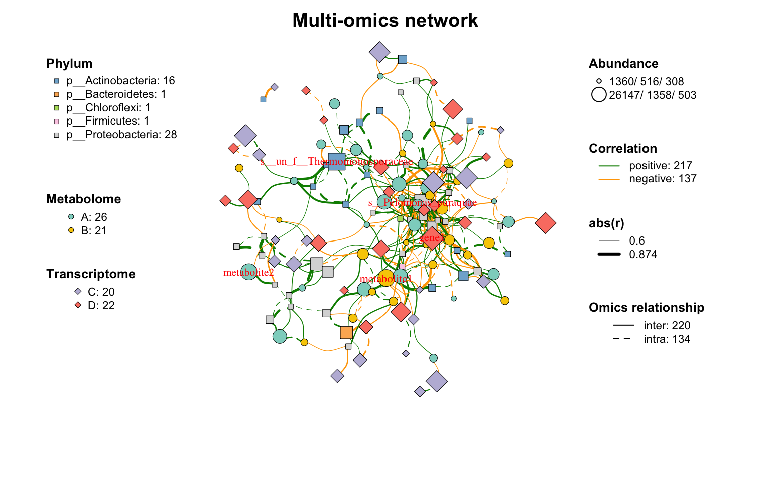
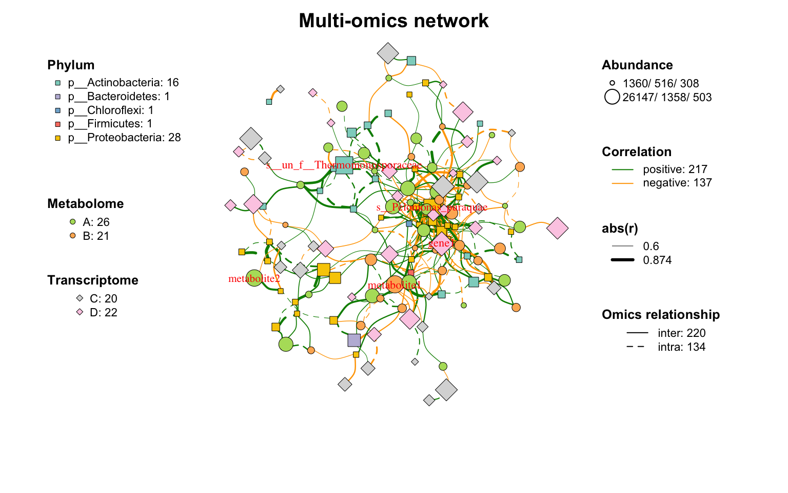
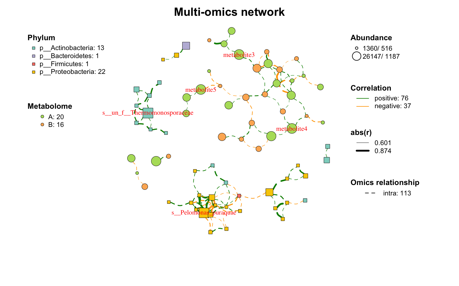
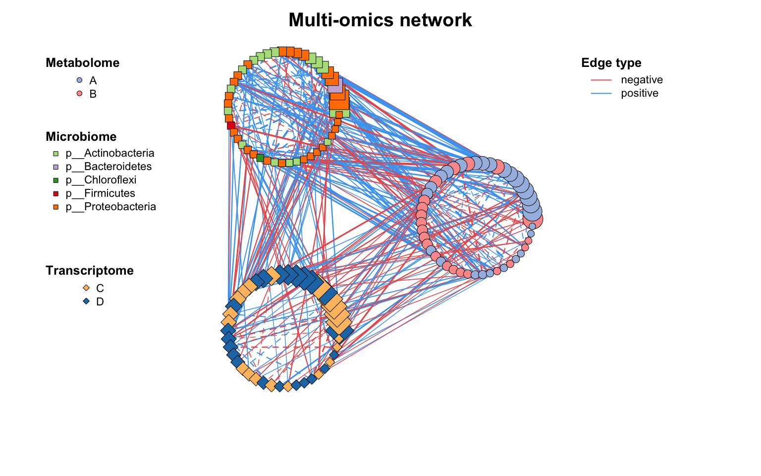
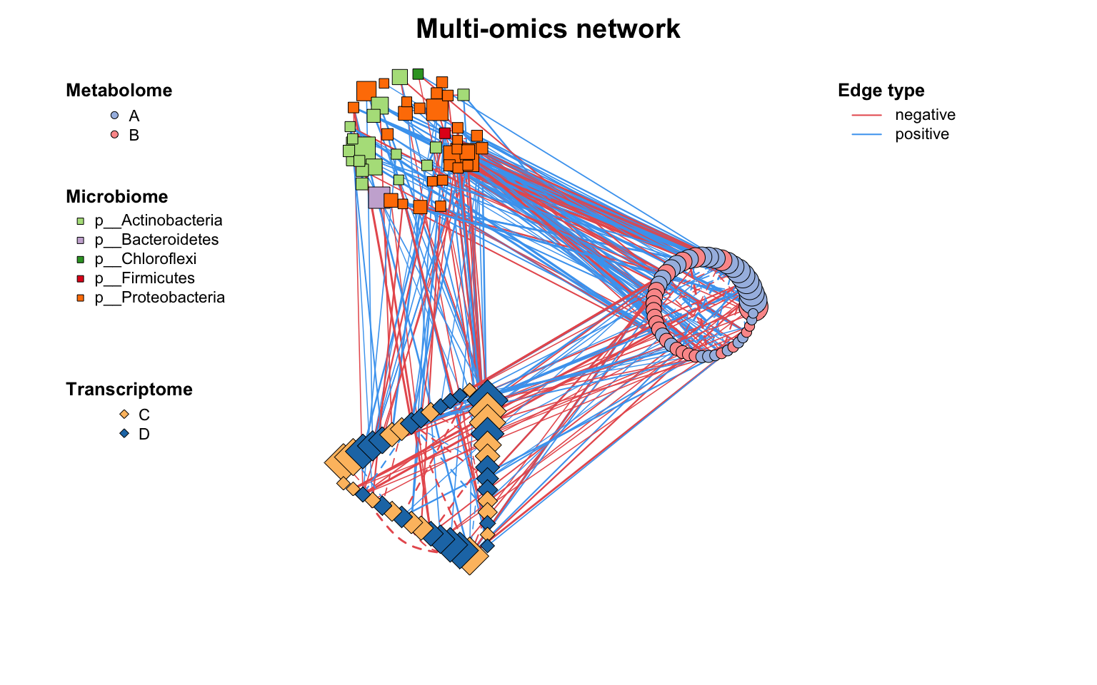
g_layout()在处理多组学网络或模块网络)时,是布局分组变量网络的极佳选择。
- 首先,指定分组变量group
- 设置组间布局
layout1,可选:- 数据框或矩阵:行名为组名,两列分别为X和Y坐标
- 函数:
c_net_layout()的各种布局方法(默认:in_circle())
- 调整
layout1的缩放比例zoom1 - 设置组内布局
layout2(使用c_net_layout()的各种布局方法), 用一个list,为每个组单独指定布局函数或者直接给一个坐标数据框。 - 调整
layout2的缩放比例zoom2,可用向量分别控制各组缩放 - 设置
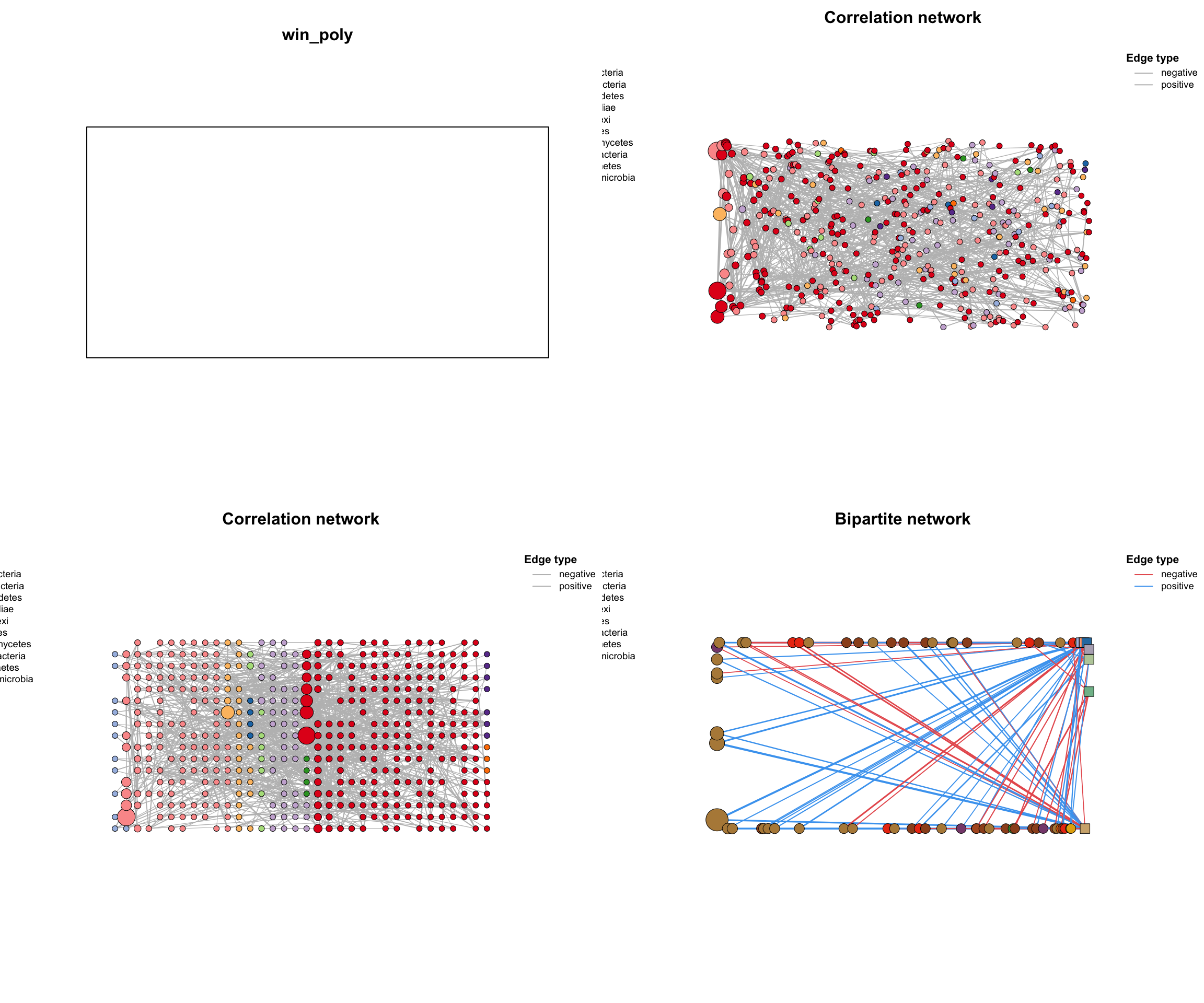
show_big_layout = T可查看layout1的分布情况
|
|
|
|
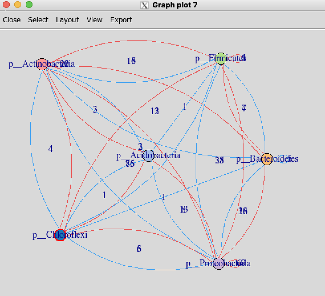
tkplot手动调整大布局
|
|
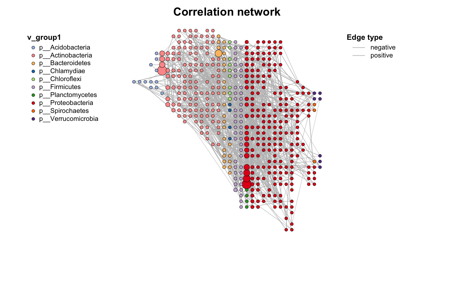
MetaNet还提供了一些预设的分组布局方法:
g_layout_circlepack()g_layout_treemap()g_layout_backbone()g_layout_stress()g_layout_polyarc()g_layout_polygon()g_layout_polycircle()g_layout_multi_layer()伪3D效果g_layout_poly_sector()
示例代码:
|
|

spatstat layout
|
|
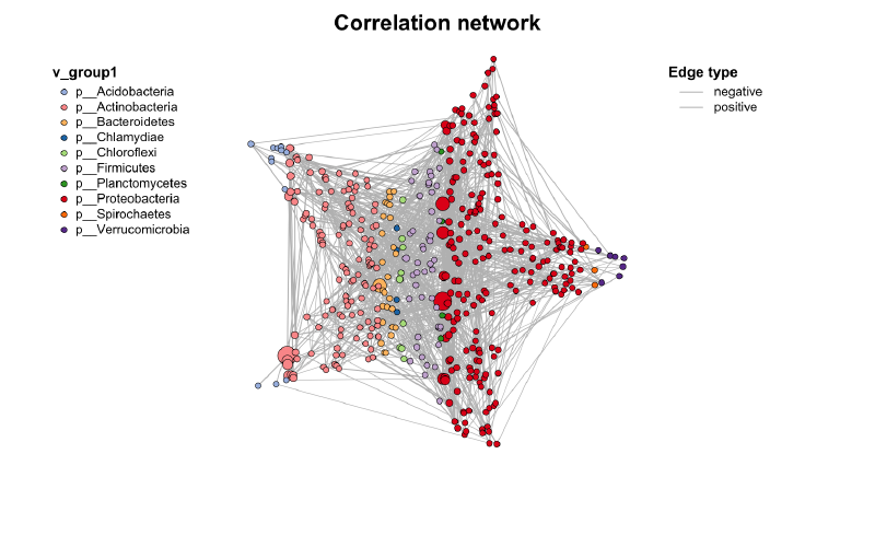
尝试画个五角星⭐️:
|
|

甚至可以画成地图:
|
|
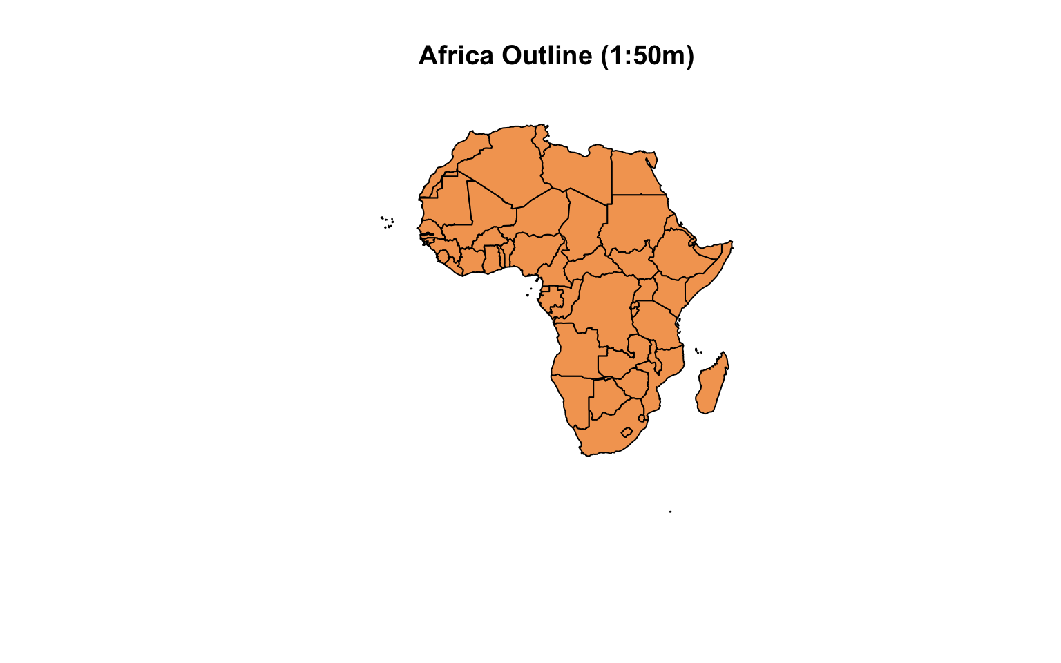
|
|
MetaNet使用的是igraph的绘图方式,R的基础绘图,所以需要用pdf,png等设备保存图片。下一节介绍MetaNet和其他绘图方式如ggplot2,D3等的转换,以及MetaNet配合Gephi,Cytoscape等交互式软件使用。
References
- Koutrouli M, Karatzas E, Paez-Espino D and Pavlopoulos GA (2020) A Guide to Conquer the Biological Network Era Using Graph Theory. Front. Bioeng. Biotechnol. 8:34. doi: 10.3389/fbioe.2020.00034
- Faust, K., and Raes, J. (2012). Microbial interactions: from networks to models. Nat. Rev. Microbiol. https://doi.org/10.1038/nrmicro2832.
- Y. Deng, Y. Jiang, Y. Yang, Z. He, et al., Molecular ecological network analyses. BMC bioinformatics (2012), doi:10.1186/1471-2105-13-113.