使用MetaNet进行网络比较

Introduction

MetaNet是一个用于组学网络分析的R包，提供了多种功能，包括网络构建、可视化、比较和稳定性分析等。

之前发布的推文中，有多位同学提到如何进行网络的比较，我也根据他们的一些建议改进了MetaNet的一些函数。本文将介绍如何使用MetaNet进行网络比较，并展示一些示例代码和结果。

软件主页：https://github.com/Asa12138/MetaNet 大家可以帮忙在github上点点star⭐️，谢谢🙏
详细英文版教程：https://bookdown.org/Asa12138/metanet_book/

可以从 CRAN 安装稳定版：install.packages("MetaNet")，本文请使用最新的开发版本。

最新的开发版本可以在 https://github.com/Asa12138/MetaNet 中找到：

1

remotes::install_github("Asa12138/MetaNet", dependencies = T)

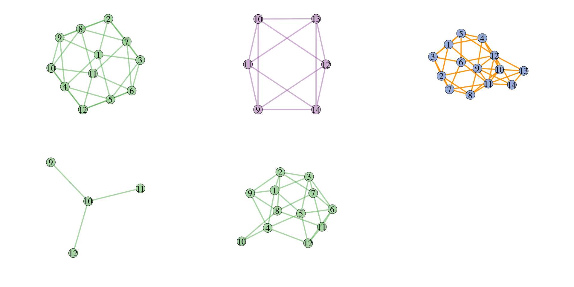
网络间运算

多个网络之间的比较和运算操作对组学数据分析很重要，例如，比较不同组别网络之间的差异部分，或者是探究动态网络变化中的核心稳定子网络。为了方便比较，MetaNet提供了c_net_union、c_net_intersect、c_net_difference等函数来计算网络的并集、交集和差集。

 1
 2
 3
 4
 5
 6
 7
 8
 9
10
11
12
13
14
15
16
17
18
19
20
21
22
23
24
25
26
27
28
29


library(MetaNet)
library(igraph)

set.seed(123)
g1 <- make_graph("Icosahedron")
V(g1)$color <- "#4DAF4A77"
E(g1)$color <- "#4DAF4A77"
g1=as.metanet(g1)

g2 <- make_graph("Octahedron")
V(g2)$name=as.character(9:14)
V(g2)$color <- "#984EA366"         # 紫色
E(g2)$color <- "#984EA366"
g2=as.metanet(g2)

# 执行操作
g_union <- c_net_union(g1, g2)
E(g_union)$color<-"orange"
g_inter <- c_net_intersect(g1, g2)
g_diff <- c_net_difference(g1, g2)

par_ls=list(main = "",legend = F,vertex_size_range = c(20,20))
par(mfrow = c(2, 3))

c_net_plot(g1, params_list = par_ls)
c_net_plot(g2, params_list = par_ls)
c_net_plot(g_union, params_list = par_ls)
c_net_plot(g_inter , params_list = par_ls)
c_net_plot(g_diff, params_list = par_ls)

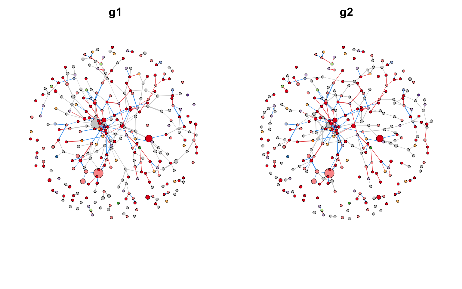
c_net_compare

基于上述的网络运算，MetaNet提供了c_net_compare函数来比较两个网络的差异部分。该函数可以计算两个网络之间的并集、交集、网络拓扑指标以及计算的网络相似性，并返回一个包含这些信息的列表。

1
2
3
4
5
6
7
8


set.seed(12)
co_net_p1=c_net_filter(co_net,name%in%sample(V(co_net)$name,300))
co_net_p2=c_net_filter(co_net,name%in%sample(V(co_net)$name,300))

c_net_compare(co_net_p1,co_net_p2)->c_net_comp

# 展示网络拓扑指标
c_net_comp$net_par_df

 1
 2
 3
 4
 5
 6
 7
 8
 9
10
11
12
13


##                                    g1            g2     g_union       g_inter
## Node_number             300.000000000 300.000000000 392.0000000 208.000000000
## Edge_number             334.000000000 321.000000000 499.0000000 156.000000000
## Edge_density              0.007447046   0.007157191   0.0065113   0.007246377
## Negative_percentage       0.443113772   0.389408100   0.4128257   0.429487179
## Average_path_length       6.801472290   6.964863184   7.3484195   5.549893086
## Global_efficiency         0.088800074   0.067651256   0.1044344   0.033600618
## Average_degree            2.226666667   2.140000000   2.5459184   1.500000000
## Average_weighted_degree   0.787061535   0.755481803   0.8992606   0.530061699
## Diameter                 18.000000000  18.000000000  19.0000000  13.000000000
## Clustering_coefficient    0.330228620   0.311132255   0.2922078   0.337595908
## Centralized_betweenness   0.127059002   0.074659531   0.1184792   0.049258854
## Natural_connectivity      3.441388267   2.895183227   4.3359822   1.643829036

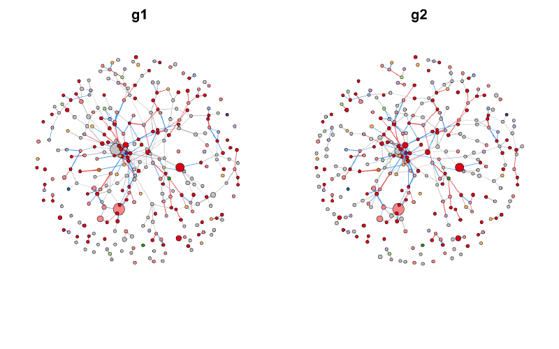
直接plot一下，结果图会将两个网络中不同的节点和边变成灰色，相当于共有节点和边高亮出来，帮助我们更好地看见网络的共有或差异部分。

1

plot(c_net_comp)

网络相似性计算了三种，一个是基于共有节点的jaccard相似性，一个是基于共有边的jaccard相似性，还有一个是基于网络邻接矩阵的相似性。

1

c_net_comp$net_similarity

1
2


##         node_jaccard         edge_jaccard adjacency_similarity 
##            0.5306122            0.3126253            0.9331847

邻接矩阵相似性计算的实现代码如下：

 1
 2
 3
 4
 5
 6
 7
 8
 9
10
11
12
13
14
15
16
17
18
19
20
21
22
23
24
25
26
27
28
29
30
31
32
33
34


adjacency_similarity <- function(g1, g2, method = "frobenius") {
  if(!is_metanet(g1)) g1 <- as.metanet(g1)
  if(!is_metanet(g2)) g2 <- as.metanet(g2)
  # 获取邻接矩阵
  adj1 <- as.matrix(igraph::as_adjacency_matrix(g1))
  adj2 <- as.matrix(igraph::as_adjacency_matrix(g2))

  # 统一节点集合
  all_nodes <- union(rownames(adj1), rownames(adj2))

  # 初始化全零矩阵
  adj1_fixed <- matrix(0, nrow = length(all_nodes), ncol = length(all_nodes),
                       dimnames = list(all_nodes, all_nodes))
  adj2_fixed <- matrix(0, nrow = length(all_nodes), ncol = length(all_nodes),
                       dimnames = list(all_nodes, all_nodes))

  # 填充已知边
  adj1_fixed[rownames(adj1), colnames(adj1)] <- adj1
  adj2_fixed[rownames(adj2), colnames(adj2)] <- adj2

  # 计算相似性
  if (method == "frobenius") {
    diff_norm <- norm(adj1_fixed - adj2_fixed, "F")
    max_norm <- sqrt(nrow(adj1_fixed) * ncol(adj2_fixed))
    similarity <- 1 - diff_norm / max_norm
  } else if (method == "cosine") {
    similarity <- sum(adj1_fixed * adj2_fixed) /
      (norm(adj1_fixed, "F") * norm(adj2_fixed, "F"))
  } else {
    stop("Method must be 'frobenius' or 'cosine'.")
  }

  return(similarity)
}

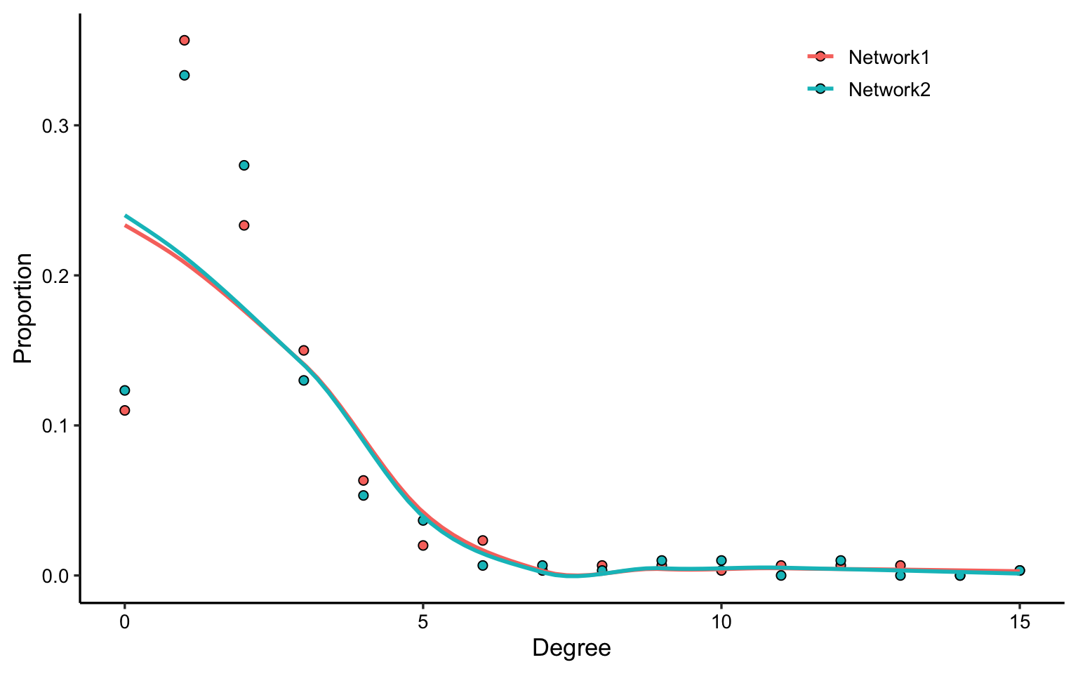
我们还可以使用plot_net_degree函数来绘制网络的度分布图，帮助更好地理解网络的结构特征，下面这两个随机取出来的子网络的度分布非常类似。

1

plot_net_degree(list(co_net_p1,co_net_p2))

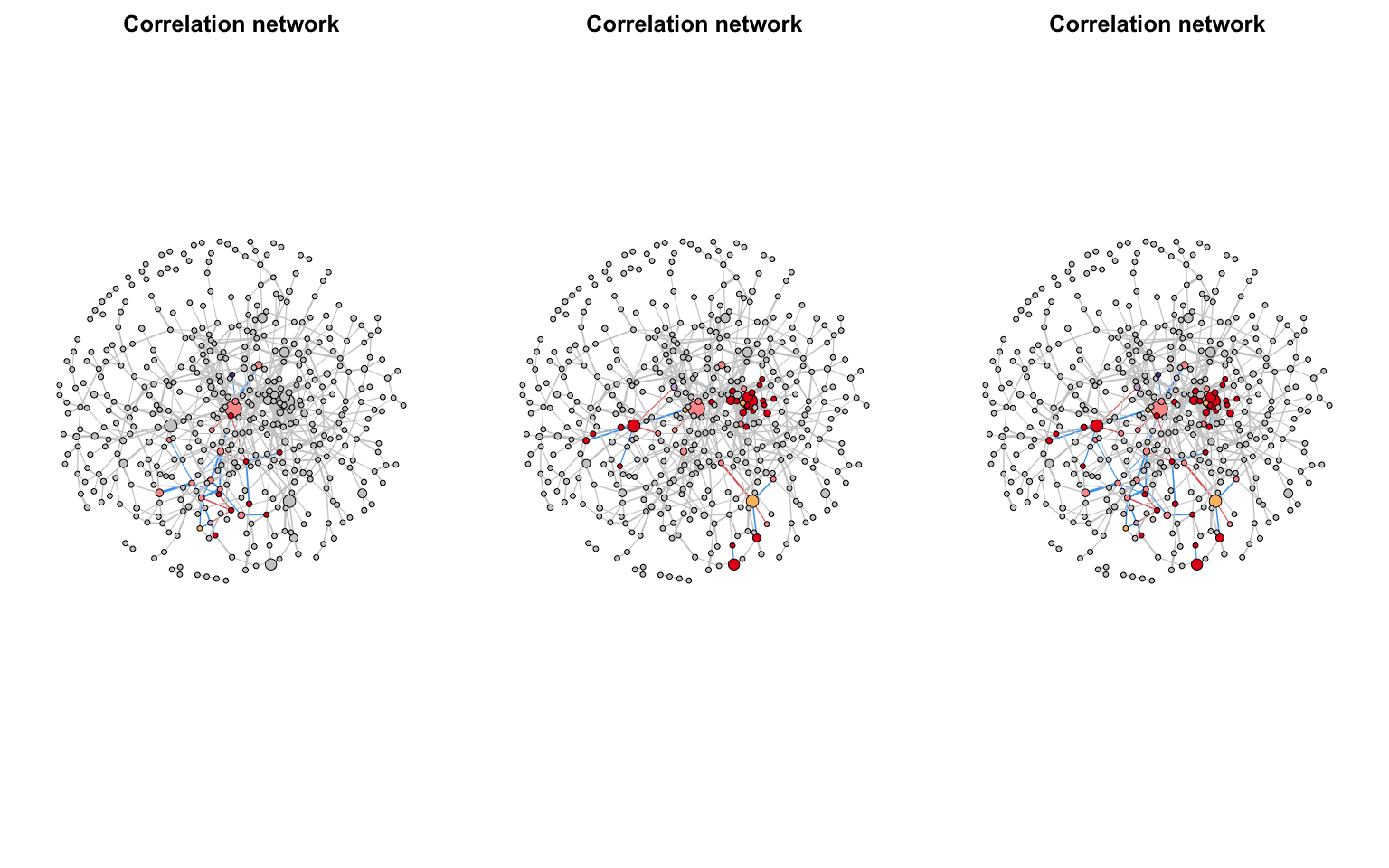
c_net_highlight

我们也可以自行调用以下这些函数：

c_net_neighbors函数可以获取指定节点的邻居节点，

c_net_highlight函数可以高亮显示网络中指定的节点和边，方便用户进行网络比较和分析。

plot_multi_nets函数可以将多个网络图并排显示，便于展示。

 1
 2
 3
 4
 5
 6
 7
 8
 9
10
11


nodes <- c("s__Kribbella_catacumbae", "s__Verrucosispora_andamanensis")
nodes <- V(c_net_neighbors(co_net, nodes, order = 2))$name

g_hl <- c_net_highlight(co_net, nodes = nodes)
get_e(co_net) %>% head(40) -> hl_edges
g_hl2 <- c_net_highlight(co_net, edges = hl_edges[, 2:3])
g_hl3 <- c_net_highlight(co_net, nodes = nodes, edges = hl_edges[, 2:3])

plot_multi_nets(
  list(g_hl, g_hl2, g_hl3),nrow = 1,multi_params_list = list(list(legend=F))
)