引言:为什么需要联合模型
在医学随访研究中,我们经常同时观察到两类数据:
- 纵向数据(Longitudinal data):同一患者在不同随访时间重复测量的生物标志物,比如血清胆红素(serBilir)、CD4 细胞计数、肿瘤标志物等。这些指标随时间动态变化。
- 生存数据(Time-to-event data):患者发生终点事件的时间,比如死亡、复发、移植等。
传统做法是"两步走"——先用线性混合模型分析纵向指标的变化,再用 Cox 比例风险模型分析生存时间。但这存在一个根本问题:纵向指标通常存在测量误差,且只在离散的随访时间点被观测到。直接把观测值当作真实值塞进 Cox 模型,会低估关联、引入偏倚。
联合模型(Joint Model)的核心思想是:用一个"潜在真实值"$\tilde{y}_i(t)$)同时驱动纵向过程和生存过程。它把纵向子模型估计出的、剔除了测量误差的真实轨迹,作为时变协变量代入生存子模型。由于两个子模型通过共享的随机效应/潜在值联系起来,故称"共享参数模型(Shared Parameter Model)"。
这样做的优势在临床动态预测中体现得最明显:医生可以基于某位患者到目前为止的纵向历史,实时估计其未来的生存概率,并且每多一次随访,预测就会更新一次。这正是"个性化、动态化"的临床决策支持。
模型设定与统计原理
1. 纵向子模型
用线性混合模型(LMM)刻画第$i$ 个患者、第$j$ 次随访的真实纵向轨迹:
$$
y_{ij} = m_i(t_{ij}) + \varepsilon_{ij} = \mathbf{x}_i^\top(t_{ij})\boldsymbol{\beta} + \mathbf{z}_i^\top(t_{ij})\mathbf{b}_i + \varepsilon_{ij}
$$其中$\boldsymbol{\beta}$ 为固定效应,$\mathbf{b}_i\sim N(0, D)$ 为个体随机效应,$\varepsilon_{ij}\sim N(0,\sigma^2)$ 为测量误差。真实轨迹$m_i(t)$ 是剔除了误差的部分。
2. 生存子模型
以相对风险(relative risk)形式,把真实轨迹作为时变协变量:
$$
h_i(t) = h_0(t)\exp\left(\boldsymbol{\gamma}^\top \mathbf{w}_i + \alpha\, m_i(t)\right)
$$其中$\mathbf{w}_i$ 是基线协变量,$h_0(t)$ 是基线风险函数,$\alpha$ 是关联参数(Association parameter)——它量化真实纵向轨迹每变化一个单位,死亡风险的变化倍数(即 hazard ratio 的对数)。
3. 关联结构(Parameterization)
$\alpha$ 到底"关联什么"有几种选择:
value(当前值):$m_i(t)$ 本身。最常用,回答"当前指标水平越高,风险越大吗"。slope(变化斜率):$\frac{d}{dt}m_i(t)$。回答"指标恶化得越快,风险越大吗"。both:同时纳入当前值和斜率。
4. 联合似然与估计
联合模型的似然是两个子模型似然的乘积,但纵向过程的随机效应$\mathbf{b}_i$ 与生存过程的终点事件相关,因此要对随机效应积分:
$$
L = \prod_{i} \int f(y_i \mid \mathbf{b}_i)\, f(T_i, \delta_i \mid \mathbf{b}_i)\, f(\mathbf{b}_i)\, d\mathbf{b}_i
$$这个积分没有解析解,JM 包用 (伪)自适应 Gauss-Hermite 求积((pseudo) adaptive Gauss-Hermite) 近似,并用 EM 算法 + 拟牛顿法优化。
5. 动态预测(Dynamic Prediction)
联合模型最有价值的地方是条件生存概率的动态预测。给定患者$i$ 在$t$ 时刻之前的所有纵向观测$\tilde{y}_i(t)$,预测其能活过$u>t$ 的概率:
$$
P(T_i > u \mid T_i > t,\ \tilde{y}_i(t),\ \mathbf{w}_i)
$$survfitJM() 用蒙特卡洛方法逼近该概率:从参数渐近正态分布抽样 → 从后验分布抽样随机效应 → 计算条件生存概率 → 多次重复求均值、中位数和置信区间。随着随访时间$t$ 后移、信息增多,预测会相应更新,这正是临床动态预测的精髓。
JM包完整操作流程
下面用 JM 包内置的 PBC(原发性胆汁性胆管炎) 数据集演示。该数据记录 312 名 PBC 患者的纵向血清胆红素(serBilir)和死亡/移植结局,是联合模型的经典教材数据。
步骤0:安装与加载包
1
2
|
# 首次使用时安装
install.packages(c("JM", "nlme", "survival", "dplyr", "ggplot2"))
|
1
2
3
4
5
|
library(JM)       # 联合模型
library(nlme)     # 线性混合模型(JM 依赖)
library(survival) # 生存模型(JM 依赖)
library(dplyr)    # 数据操作
library(ggplot2)  # 可视化
|
步骤1:了解数据结构
1
2
|
data(pbc2)     # 纵向数据:每患者多行
data(pbc2.id)  # 生存数据:每患者一行
|
 1
 2
 3
 4
 5
 6
 7
 8
 9
10
11
12
13
14
15
16
17
18
19
20
21
22
23
24
25
26
27
28
|
# 纵向数据结构(同一 id 有多次随访)
head(pbc2)
##   id    years status      drug      age    sex      year ascites hepatomegaly
## 1  1  1.09517   dead D-penicil 58.76684 female 0.0000000     Yes          Yes
## 2  1  1.09517   dead D-penicil 58.76684 female 0.5256817     Yes          Yes
## 3  2 14.15234  alive D-penicil 56.44782 female 0.0000000      No          Yes
## 4  2 14.15234  alive D-penicil 56.44782 female 0.4983025      No          Yes
## 5  2 14.15234  alive D-penicil 56.44782 female 0.9993429      No          Yes
## 6  2 14.15234  alive D-penicil 56.44782 female 2.1027270      No          Yes
##   spiders                   edema serBilir serChol albumin alkaline  SGOT
## 1     Yes edema despite diuretics     14.5     261    2.60     1718 138.0
## 2     Yes edema despite diuretics     21.3      NA    2.94     1612   6.2
## 3     Yes                No edema      1.1     302    4.14     7395 113.5
## 4     Yes                No edema      0.8      NA    3.60     2107 139.5
## 5     Yes                No edema      1.0      NA    3.55     1711 144.2
## 6     Yes                No edema      1.9      NA    3.92     1365 144.2
##   platelets prothrombin histologic status2
## 1       190        12.2          4       1
## 2       183        11.2          4       1
## 3       221        10.6          3       0
## 4       188        11.0          3       0
## 5       161        11.6          3       0
## 6       122        10.6          3       0
cat("\n纵向数据集:", nrow(pbc2), "行,", length(unique(pbc2$id)), "位患者\n")
##
## 纵向数据集: 1945 行, 312 位患者
cat("随访时间范围(years):", range(pbc2$years), "\n")
## 随访时间范围(years): 0.112255 14.30566
|
 1
 2
 3
 4
 5
 6
 7
 8
 9
10
11
12
|
# 生存数据结构
head(pbc2.id[, c("id", "years", "status2", "drug")])
##   id     years status2      drug
## 1  1  1.095170       1 D-penicil
## 2  2 14.152338       0 D-penicil
## 3  3  2.770781       1 D-penicil
## 4  4  5.270507       1 D-penicil
## 5  5  4.120578       0   placebo
## 6  6  6.853028       1   placebo
cat("\n事件数(status2=1):", sum(pbc2.id$status2), " / ", nrow(pbc2.id), "\n")
##
## 事件数(status2=1): 140  /  312
|
要点:pbc2 是长格式的纵向数据(years 是随访时间),pbc2.id 是每人一行的生存数据(years 是事件/删失时间,status2 是事件指示变量)。联合模型需要这两份数据。**
步骤2:拟合两个子模型
 1
 2
 3
 4
 5
 6
 7
 8
 9
10
11
12
13
14
15
16
17
18
19
20
21
22
23
24
25
26
27
28
29
30
31
32
33
34
35
36
37
38
39
40
41
|
# 纵向子模型:log-胆红素 ~ 药物 * 时间,随机斜率(允许每人变化速度不同)
lmeFit <- lme(log(serBilir) ~ drug * year,
              random = ~ year | id,
              data = pbc2)

# 生存子模型:必须指定 x = TRUE(jointModel 需要设计矩阵)
survFit <- coxph(Surv(years, status2) ~ drug,
                 data = pbc2.id, x = TRUE)

summary(lmeFit)
## Linear mixed-effects model fit by REML
##   Data: pbc2
##        AIC      BIC    logLik
##   3085.474 3130.042 -1534.737
##
## Random effects:
##  Formula: ~year | id
##  Structure: General positive-definite, Log-Cholesky parametrization
##             StdDev    Corr
## (Intercept) 0.9985874 (Intr)
## year        0.1722100 0.417
## Residual    0.3489329
##
## Fixed effects:  log(serBilir) ~ drug * year
##                         Value  Std.Error   DF   t-value p-value
## (Intercept)         0.5630314 0.08255263 1631  6.820272  0.0000
## drugD-penicil      -0.1332474 0.11610817  310 -1.147614  0.2520
## year                0.1797540 0.01782101 1631 10.086633  0.0000
## drugD-penicil:year -0.0044099 0.02490438 1631 -0.177074  0.8595
##  Correlation:
##                    (Intr) drgD-p year
## drugD-penicil      -0.711
## year                0.248 -0.176
## drugD-penicil:year -0.177  0.251 -0.716
##
## Standardized Within-Group Residuals:
##         Min          Q1         Med          Q3         Max
## -4.32411085 -0.49870809 -0.01666735  0.45288335  5.28785685
##
## Number of Observations: 1945
## Number of Groups: 312
|
步骤3:拟合联合模型
 1
 2
 3
 4
 5
 6
 7
 8
 9
10
11
12
13
14
15
16
17
18
19
20
21
22
23
24
25
26
27
28
29
30
31
32
33
34
35
36
37
38
39
40
41
42
43
44
45
46
47
48
49
50
|
set.seed(8314)
jointFit <- jointModel(lmeFit, survFit, timeVar = "year")

summary(jointFit)
##
## Call:
## jointModel(lmeObject = lmeFit, survObject = survFit, timeVar = "year")
##
## Data Descriptives:
## Longitudinal Process		Event Process
## Number of Observations: 1945	Number of Events: 140 (44.9%)
## Number of Groups: 312
##
## Joint Model Summary:
## Longitudinal Process: Linear mixed-effects model
## Event Process: Weibull relative risk model
## Parameterization: Time-dependent
##
##    log.Lik      AIC      BIC
##  -1918.529 3861.058 3905.974
##
## Variance Components:
##              StdDev    Corr
## (Intercept)  1.0003  (Intr)
## year         0.1807  0.4244
## Residual     0.3471
##
## Coefficients:
## Longitudinal Process
##                      Value Std.Err z-value p-value
## (Intercept)         0.5594  0.0827  6.7653 <0.0001
## drugD-penicil      -0.1334  0.1162 -1.1483  0.2509
## year                0.1865  0.0189  9.8835 <0.0001
## drugD-penicil:year -0.0038  0.0255 -0.1506  0.8803
##
## Event Process
##                 Value Std.Err  z-value p-value
## (Intercept)   -4.4038  0.2734 -16.1065 <0.0001
## drugD-penicil  0.0377  0.1799   0.2095  0.8340
## Assoct         1.2396  0.0931  13.3196 <0.0001
## log(shape)     0.0177  0.0828   0.2139  0.8306
##
## Scale: 1.0179
##
## Integration:
## method: (pseudo) adaptive Gauss-Hermite
## quadrature points: 5
##
## Optimization:
## Convergence: 0
|
结果解读
输出分三块:
- 纵向过程(Longitudinal Process):与单独的
lme 结果一致。year 显著(p<0.001)说明胆红素随时间上升;drugD-penicil:year 不显著说明青霉胺未显著改变胆红素上升速率。
- 事件过程(Event Process):这是联合模型的核心。
drugD-penicil:药物对生存的直接效应,不显著。Assoct = 1.24,p < 0.001:关联参数$\alpha$。表示真实胆红素水平每升高 log 单位,死亡风险增加到$e^{1.24} \approx 3.45$ 倍。这是剔除了测量误差后的真实关联,比直接把观测值塞进 Cox 模型更可靠。log(shape):Weibull 基线风险的形状参数。
- 方差成分(Variance Components):随机截距和随机斜率的方差及相关性。
注意:Assoct 正是联合模型区别于"两步法"的关键——它用的是潜在真实值$m_i(t)$,而不是含误差的观测值。
步骤4:动态预测——单个患者
假设患者 12 号已经随访到第 10 年,我们要预测他之后还能活多久。取他在$t=10$ 之前的所有纵向历史。
1
2
3
4
5
6
7
8
|
# 患者 12 的纵向历史
ND <- pbc2[pbc2$id == "12", ]
nrow(ND)  # 已测次数
## [1] 2
tail(ND[, c("years", "serBilir")])
##        years serBilir
## 70 0.8323294      3.6
## 71 0.8323294     10.0
|
 1
 2
 3
 4
 5
 6
 7
 8
 9
10
11
12
13
14
15
16
17
18
19
20
21
|
# 在 t0=10 时刻做动态预测
sfit <- survfitJM(jointFit, newdata = ND, idVar = "id", last.time = 10)
sfit
##
## Prediction of Conditional Probabilities of Event
## 	based on 200 Monte Carlo samples
##
## $`12`
##      times   Mean Median  Lower  Upper
## 1  10.0000 1.0000 1.0000 1.0000 1.0000
## 1  10.2017 0.9405 0.9585 0.7923 0.9965
## 2  10.6221 0.8324 0.8745 0.4677 0.9897
## 3  11.0425 0.7424 0.7964 0.2594 0.9834
## 4  11.4629 0.6671 0.7225 0.1343 0.9776
## 5  11.8833 0.6038 0.6521 0.0644 0.9722
## 6  12.3037 0.5501 0.5843 0.0283 0.9672
## 7  12.7241 0.5043 0.5206 0.0113 0.9625
## 8  13.1445 0.4650 0.4612 0.0041 0.9582
## 9  13.5649 0.4310 0.4065 0.0013 0.9542
## 10 13.9853 0.4013 0.3592 0.0004 0.9505
## 11 14.4057 0.3754 0.3161 0.0001 0.9471
|
输出中 Mean 是该患者未来各时间点的条件生存概率(默认基于 200 次蒙特卡洛抽样)。比如第 10 年时点概率为 1(因为已知活到 10 年),到第 11 年降到约 0.74,第 14 年约 0.40。
步骤5:可视化动态预测
survfitJM() 的 summaries 是列表,每个元素是一张矩阵,列含 times、Mean、Median、Lower、Upper。我们用 ggplot2 画出条件生存曲线及置信带。
 1
 2
 3
 4
 5
 6
 7
 8
 9
10
|
# 把 summaries 转成 data.frame(summaries[[1]] 是矩阵)
pred <- as.data.frame(sfit$summaries[[1]])

ggplot(pred, aes(x = times, y = Mean)) +
  geom_line(linewidth = 1, color = "#2c7fb8") +
  geom_ribbon(aes(ymin = Lower, ymax = Upper), alpha = 0.2, fill = "#2c7fb8") +
  geom_vline(xintercept = 10, linetype = 2, color = "grey40") +
  labs(x = "Years since baseline", y = "Conditional survival probability",
       title = "Dynamic prediction: Patient 12 (known alive until t=10)") +
  theme_minimal()
|
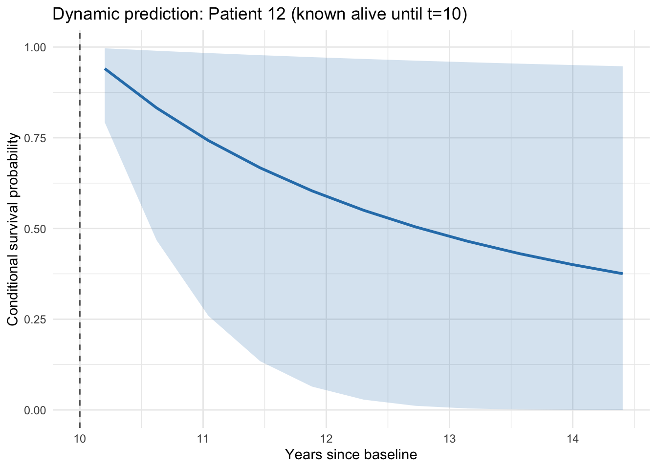
动态预测的意义:竖虚线是预测起点$t=10$。曲线从 1.0 开始下降,反映"已知该患者活到第 10 年"这一条件。随着更多随访数据收集,重新调用 survfitJM() 即可得到更新后的预测。
步骤6:同一患者、不同预测起点的对比(体现"信息越多越精准")
下面演示"动态"二字——同一位患者,分别在只随访到 6 年和随访到 10 年时做预测,看看预测如何随信息量改变。
 1
 2
 3
 4
 5
 6
 7
 8
 9
10
11
12
13
14
15
16
17
18
|
pred_list <- list()

for (t0 in c(6, 10)) {
  set.seed(8314)
  s <- survfitJM(jointFit, newdata = ND, idVar = "id", last.time = t0, M = 100)
  df_s <- as.data.frame(s$summaries[[1]])
  df_s$pred_at <- paste0("Predicted at t0 = ", t0, "y")
  pred_list[[as.character(t0)]] <- df_s
}

pred_all <- bind_rows(pred_list)

ggplot(pred_all, aes(x = times, y = Mean, color = pred_at)) +
  geom_line(linewidth = 1) +
  labs(x = "Years since baseline", y = "Conditional survival probability",
       title = "Same patient, more follow-up = updated prediction",
       color = "Prediction time") +
  theme_minimal()
|
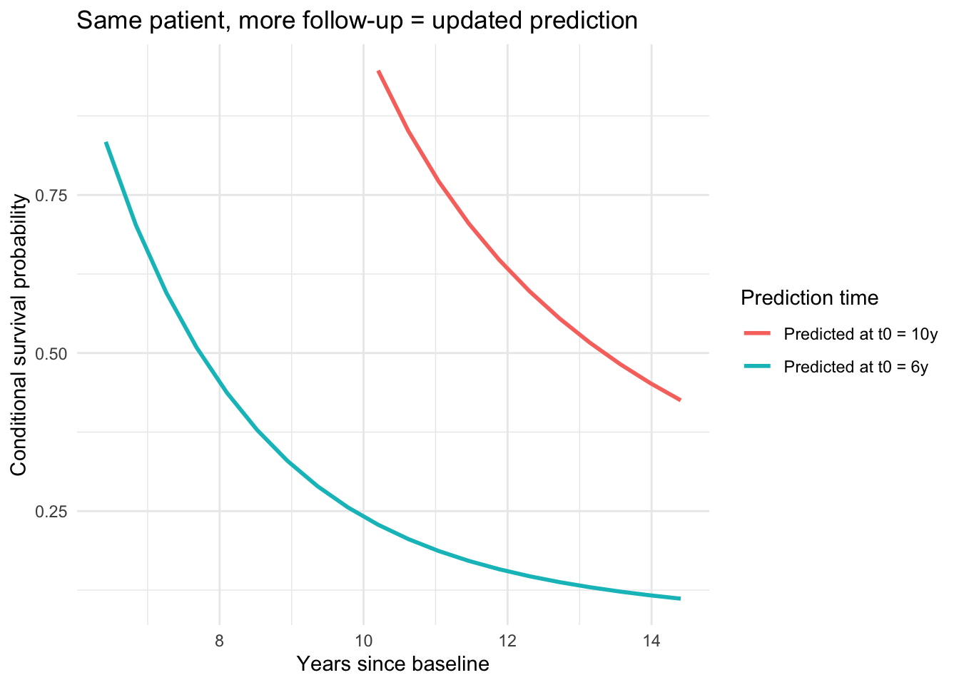
可以观察到:随访到 10 年时(红色)的预测整体高于只随访到 6 年时(蓝绿)的预测——因为到第 10 年患者仍然存活,这一额外信息让条件生存概率整体上移。这就是动态更新。
步骤7:多位患者的联合预测(临床队列应用)
临床中常要对一批患者同时做风险分层。可以用一个循环对多个患者分别预测,并画出各自的条件生存曲线。
 1
 2
 3
 4
 5
 6
 7
 8
 9
10
11
12
13
14
15
16
17
18
|
# 示例:对患者 10、12 在各自最后观测时间做动态预测
ids <- c("10", "12")
pred_multi <- list()
for (id in ids) {
  set.seed(8314)
  s <- survfitJM(jointFit, newdata = pbc2[pbc2$id == id, ],
                 idVar = "id", last.time = tail(pbc2$years[pbc2$id == id], 1), M = 100)
  df_s <- as.data.frame(s$summaries[[1]])
  df_s$subject <- paste0("Patient ", id)
  pred_multi[[id]] <- df_s
}
pred_multi <- bind_rows(pred_multi)

ggplot(pred_multi, aes(x = times, y = Mean, color = subject)) +
  geom_line(linewidth = 1) +
  labs(x = "Years since baseline", y = "Conditional survival probability",
       title = "Dynamic prediction for multiple patients", color = "Subject") +
  theme_minimal()
|
步骤8:模型选择与敏感性
联合模型本身可以作为预测工具,也可以通过似然比/AIC 在多种设定之间比较:
parameterization:value / slope / both。method:基线风险的假设,weibull-PH-aGH(默认)、piecewise-PH-aGH(分段常值,更灵活)、spline-PH-aGH(样条)等。
下面比较不同基线风险设定:
 1
 2
 3
 4
 5
 6
 7
 8
 9
10
11
12
13
14
|
set.seed(8314)
fit_wb <- jointModel(lmeFit, survFit, timeVar = "year", method = "weibull-PH-aGH")
set.seed(8314)
fit_pw <- jointModel(lmeFit, survFit, timeVar = "year", method = "piecewise-PH-aGH")

data.frame(
  method = c(fit_wb$method, fit_pw$method),
  logLik = c(logLik(fit_wb), logLik(fit_pw)),
  AIC    = c(AIC(fit_wb),    AIC(fit_pw)),
  BIC    = c(BIC(fit_wb),    BIC(fit_pw))
)
##            method    logLik      AIC      BIC
## 1   weibull-PH-GH -1918.529 3861.058 3905.974
## 2 piecewise-PH-GH -1915.683 3865.365 3928.996
|
1
2
3
4
5
6
|
# slope/both 参数化需额外指定 derivForm(对应纵向模型对时间的导数)
# 固定效应需按设计矩阵的列号指定;此处只作示意
# df <- list(fixed = ~ drug + year, indFixed = 3:4, random = ~ year, indRandom = 2)
# set.seed(8314)
# jointFit2 <- jointModel(lmeFit, survFit, timeVar = "year",
#                         parameterization = "both", derivForm = df)
|
一般选择 AIC 较小的设定。若各设定下$\alpha$ 的方向和显著性与结论一致,说明结果对模型形式稳健。
临床预测模型的评估(进阶)
动态预测模型需要专门的评估指标,常用动态 AUC 和 Brier 分数,用来回答"这套动态预测在时间$t$ 区分高危/低危患者的能力如何"。“这里更严谨的动态 AUC 可用 riskRegression 或 JMbayes2 等包配合实现。属于进阶内容,感兴趣可自行扩展。
联合模型的优缺点
优点
- 更准确的关联估计:用潜在真实值而非含误差的观测值,避免回归稀释(regression dilution)偏倚。
- 真正的动态个性化预测:随时更新,随随访信息量提升而更精准,适合临床决策支持。
- 同时刻画两个过程:纵向轨迹 + 生存风险,一次建模获得两种信息。
- 处理信息性删失:纵向缺失/删失如果与终点事件相关,联合模型能给出更可靠的推断。
局限性
- 计算复杂、速度慢:需要对随机效应积分,样本大/随机效应维度高时很耗时。
- 模型设定敏感:纵向子模型(线性/非线性)、随机效应结构、基线风险形式都需要仔细选择。
- 对分布假设敏感:纵向响应通常假设正态;非正态需改用 GLMM 等。
- 收敛问题:复杂设定下 EM/优化可能不收敛,需检查
Convergence 标志。
- 未观测混杂依旧无法处理:与普通生存模型一样,无法平衡未测量的混杂因素。
注意事项
- 拟合前务必检查纵向子模型和生存子模型是否合理(残差、比例风险假设等)。
- 生存子模型的
coxph() 或 survreg() 必须加 x = TRUE,否则 jointModel() 报错。
- 动态预测时
newdata 必须是该患者的纵向历史(pbc2 子集),且含 idVar 指定的 ID 列。
- 用
set.seed() 保证蒙特卡洛预测和优化可重复。
- 预测结果应附上置信区间(
Lower/Upper)并说明是条件概率。
参考文献与扩展
- Rizopoulos, D. (2012). Joint Models for Longitudinal and Time-to-Event Data: with Applications in R. Chapman & Hall/CRC. (JM 包官方参考书)
- Rizopoulos, D. (2010). JM: An R Package for the Joint Modelling of Longitudinal and Time-to-Event Data. Journal of Statistical Software, 35(9), 1-33.
- Rizopoulos, D. (2011). Dynamic predictions and prospective accuracy in joint models for longitudinal and time-to-event data. Biometrics, 67, 819-829.
- 进阶/新包:
JMbayes2(贝叶斯联合模型,支持更灵活设定与动态 AUC、Brier 分数评估)、bamlss、INLA 等。
小结
联合模型把纵向生物标志物与生存时间统一建模,用潜在真实值连接两个过程,从而给出剔除了测量误差的关联估计和可随随访动态更新的个性化生存预测。本文用 R 的 JM 包 + PBC 数据走通了完整流程:拟合子模型 → 联合建模 → 解读关联参数$\alpha$ → 动态预测 → 可视化 → 模型比较。掌握这些,你就能在自己的随访数据上构建临床动态预测模型。