Featured image of post R语言实现多组学因子分析(MOFA)

R语言实现多组学因子分析(MOFA)

多组学因子分析(Multi-Omics Factor Analysis, MOFA)是一种无监督地整合多组学数据、从共享与组特异性变异中提取潜在因子的统计方法。本文用 R 的 MOFA2 包系统讲解原理与实操。

引言:为什么需要多组学因子分析

随着高通量测序技术的发展,同一批样本往往同时测了多种组学数据:转录组(RNA-seq)甲基化(DNA methylation)蛋白质组(proteomics)代谢组(metabolomics) 等。这些数据从不同层次刻画同一群样本,称之为多组学数据(multi-omics data)

多组学数据的核心价值在于"信息互补":转录组反映基因表达,甲基化反映表观调控,蛋白组反映最终功能分子。单独分析某一种组学往往只能看到"一角",而整合起来才能还原完整的生物学图景。

但整合多组学面临两大难题:

  1. 维度灾难:每种组学都有成千上万个特征(基因、位点、蛋白),远超样本数。
  2. 组学间异质性:不同组学的数据分布、量纲、噪声结构完全不同,不能简单拼接后直接跑 PCA。

多组学因子分析(Multi-Omics Factor Analysis, MOFA) 就是为解决这两个问题而生的无监督方法。它把多种组学作为"多个视图(view)",从中分解出共享的潜因子(latent factors),既能降维、又能揭示组学间共享与组特异性的生物学信号。

MOFA 最初由 Argelaguet 等人提出(Nature Methods 2018),2020 年升级为 MOFA+,支持多组(multi-group)结构。R 中的实现是 MOFA2 包,官方文档见 https://biofam.github.io/MOFA2/

MOFA 的核心原理:概率矩阵分解

1. 从单组学 PCA 到多组学 MOFA

先回顾 PCA。对单组学矩阵 $\mathbf{X}$($N$ 个样本 × $D$ 个特征),PCA 把它近似分解为:

$$ \mathbf{X} \approx \mathbf{Z}\mathbf{W}^\top $$

其中 $\mathbf{Z}$ 是 $N\times K$ 的因子得分(factor scores)(也叫潜变量),$\mathbf{W}$ 是 $D\times K$ 的载荷(loadings),$K$ 是因子数。因子得分是每个样本在新坐标下的位置,载荷是每个特征对因子的贡献。

MOFA 把同样的思想推广到多组学:假设有 $M$ 个视图(组学),第 $m$ 个视图的观测矩阵 $\mathbf{X}_m$($N$ 样本 × $D_m$ 特征)共享同一个因子得分矩阵 $\mathbf{Z}$,但每个视图有自己的载荷矩阵 $\mathbf{W}_m$:

$$ \mathbf{X}_m \approx \mathbf{Z}\mathbf{W}_m^\top + \boldsymbol{\varepsilon}_m $$

关键点在于 $\mathbf{Z}$ 是共享的——所有组学都投影到同一组潜因子上。于是 MOFA 找到的因子,代表跨组学的共同变异模式。如果某个因子只在部分组学中有信号,则对应的载荷 $\mathbf{W}_m$ 在该组学中趋近于 0。

2. 概率模型:MOFA 的完整生成模型

MOFA 是概率模型(概率矩阵分解的贝叶斯版本),把观测看作是潜因子通过载荷映射,再叠加上噪声:

$$ \mathbf{X}_m = \mathbf{Z}\mathbf{W}_m^\top + \boldsymbol{\varepsilon}_m, \qquad \boldsymbol{\varepsilon}_m \sim N(0, \boldsymbol{\Sigma}_m) $$

其中:

  • 因子得分 $\mathbf{Z}$ 服从先验 $\mathbf{Z} \sim N(0, \mathbf{I})$;
  • 载荷 $\mathbf{W}_m$ 上的先验是自动相关性判定(Automatic Relevance Determination, ARD)——每个因子在每个视图上有一个精度参数 $\alpha_{km}$。如果某因子对某视图不重要,$\alpha$ 会变大,把载荷收缩到 0,从而实现视图稀疏性(即因子只在相关组学中有载荷)。

3. ARD 先验与因子稀疏性

ARD 是 MOFA 的核心机制。每个载荷矩阵元素有先验:

$$ w_{dm} \sim N(0, \alpha_{km}^{-1}), \qquad \alpha_{km} \sim \text{Gamma}(a_0, b_0) $$

$\alpha_{km}$ 是该因子-视图组合的精度参数,通过变分推断学习。若某因子在某视图不重要,$\alpha_{km}$ 会变得很大,强迫 $w_{dm}\to 0$。这正是 MOFA 能自动实现"因子只在部分组学中活跃“的原因。

4. MOFA+ 的多组扩展

MOFA+(MOFA2 支持)进一步允许**多组(multi-group)**结构:样本可以来自不同批次、不同队列或不同条件。此时因子得分变为 $\mathbf{Z}_{gk}$,即每个 group 有自己的因子值,但共享载荷结构:

$$ \mathbf{X}_{gm} = \mathbf{Z}_{gk}\mathbf{W}_{km}^\top + \boldsymbol{\varepsilon}_{gm} $$

这意味着 MOFA 能区分共享因子(在所有组中都活跃)与组特异因子(只在某组中活跃)。这正是教学演示图里看到的:Factor2 只在 Disease 组有信号。

5. 似然与推断

给定各组学观测,模型的完全似然为:

$$ \log p(\mathbf{X} \mid \mathbf{Z}, \mathbf{W}) = \sum_m \log p(\mathbf{X}_m \mid \mathbf{Z}, \mathbf{W}_m) $$

由于是贝叶斯模型,MOFA 通过变分推断(Variational Inference) 最大化证据下界(ELBO, Evidence Lower Bound) 来近似后验。ELBO 是训练收敛的判据,也用于模型比较(因子数选择)。

MOFA2 的后端实现是 Python 包 mofapy2,R 的 run_mofa() 通过 reticulate 调用它进行优化。

MOFA 与其它整合方法的区别

方法 核心思想 适用场景 特点
MOFA 概率矩阵分解 + ARD 稀疏 多种组学、可分组 因子可跨组学解释,支持多组,可做下游关联分析
iCluster 联合潜变量聚类 基因+拷贝数等 侧重于聚类发现亚型
NMF 非负矩阵分解 单一组学表达矩阵 非负约束,解释为共表达模块
sMBPLS 多块偏最小二乘 有监督关联 需要先验的响应变量
JIVE 联合+个体变异分解 两组学对齐样本 区分共享与特异成分,但不能分组

MOFA 的相对优势在于:无监督(无需标签)、组学间权重可解释(ARD 稀疏)、支持多组结构(MOFA+)、输出可直接用于下游统计(因子值与协变量关联)。

环境准备:安装 MOFA2 与 Python 后端

MOFA2 是 Bioconductor 包,安装时需要同时安装它的 Python 后端 mofapy2

1
2
3
4
5
6
7
8
9
# 1. 安装 R 包 MOFA2
if (!requireNamespace("BiocManager", quietly = TRUE)) install.packages("BiocManager")
BiocManager::install("MOFA2")

# 2. 安装 Python 后端 mofapy2(MOFA2 用 reticulate 调用它拟合模型)
#    推荐用 conda 创建一个 Python 3.9 环境(mofapy2 目前对较新 Python 兼容性更好)
# conda create -n mofa python=3.9
# conda activate mofa
# pip install mofapy2
1
2
3
library(MOFA2)
library(dplyr)
library(ggplot2)

重要run_mofa() 需要调用 Python 的 mofapy2,因此必须让 R 的 reticulate 指向装有该模块的 Python 环境。有两种方式:

  • reticulate::use_condaenv("mofa", required = TRUE) 指定 conda 环境;
  • 或在 R 启动前设置环境变量 Sys.setenv(RETICULATE_PYTHON = "/路径/python")

若已装 basilisk 且想自动管理环境,可调用 run_mofa(..., use_basilisk = TRUE),但更推荐显式指定 Python 环境以便复现。

MOFA 完整操作流程

下面用 MOFA2 内置的 make_example_data() 合成一份三组学演示数据(RNA / 甲基化 / 蛋白),样本分成两组(Healthy / Disease)。合成数据的好处是可复现、无需下载,且真实结构已知,便于理解因子含义。真实数据的替换方式见文末。

步骤0:加载包并设定随机种子

1
2
3
4
5
library(MOFA2)
library(dplyr)
library(ggplot2)

set.seed(7841)   # 保证可复现

步骤1:准备多组学数据

MOFA2 要求数据是一个 list,每个元素是一个组学视图的矩阵,行是特征(features),列是样本(samples)。所有视图必须共享同一批样本且样本顺序一致

我们用 make_example_data() 生成 3 个视图、2 组各 60 个样本、真实含 4 个潜在因子的数据:

 1
 2
 3
 4
 5
 6
 7
 8
 9
10
11
12
13
14
15
16
17
18
19
20
21
22
23
24
# 生成合成多组学数据:3 个视图,2 组样本,真实含 4 个因子
dt <- make_example_data(
  n_views = 3, n_features = 100, n_samples = 60,
  n_groups = 2, n_factors = 4, likelihood = "gaussian"
)

data_list <- dt$data          # 视图矩阵列表
names(data_list) <- c("RNA", "DNAme", "Protein")   # 给视图起名

# 给特征加前缀,便于后续解读载荷
for (i in seq_along(data_list)) {
  rownames(data_list[[i]]) <- paste0(names(data_list)[i], "_", seq_len(nrow(data_list[[i]])))
}

# 查看每个视图的维度(特征 × 样本)
data_list |> lapply(dim)
## $RNA
## [1] 100 120
## 
## $DNAme
## [1] 100 120
## 
## $Protein
## [1] 100 120

make_example_data 的内部逻辑是:先生成真实的因子得分 $\mathbf{Z}$ 和载荷 $\mathbf{W}$,再用它们乘出无噪声信号并加观测噪声。这样我们知道因子"真相”,方便验证 MOFA 能否找回它们。

样本元数据create_mofa() 需要样本分组信息。我们构造一个包含 group 和协变量 disease 的元数据框:

 1
 2
 3
 4
 5
 6
 7
 8
 9
10
11
12
13
14
15
16
17
18
n <- ncol(data_list$RNA)   # 120 个样本

samples_meta <- data.frame(
  sample  = colnames(data_list$RNA),
  group   = rep(c("Healthy", "Disease"), each = n / 2),
  disease = rep(rep(c("Control", "Case"), each = n / 4), 2),
  stringsAsFactors = FALSE
)

# 检查样本数与分组
table(samples_meta$group)
## 
## Disease Healthy 
##      60      60
table(samples_meta$disease)
## 
##    Case Control 
##      60      60

要点:元数据的行顺序必须与数据矩阵的列顺序完全一致make_example_data 已经保证了这点,但用真实数据时务必自行核对。

步骤2:创建 MOFA 对象

 1
 2
 3
 4
 5
 6
 7
 8
 9
10
11
12
13
14
15
# 创建 MOFA 对象,指定视图列表与分组
mofa <- create_mofa(data_list, groups = samples_meta$group)

# 挂载样本元数据(用于后续按协变量着色、关联分析)
samples_metadata(mofa) <- samples_meta

mofa
## Untrained MOFA model with the following characteristics: 
##  Number of views: 3 
##  Views names: RNA DNAme Protein 
##  Number of features (per view): 100 100 100 
##  Number of groups: 2 
##  Groups names: Disease Healthy 
##  Number of samples (per group): 60 60 
## 

这一步只是把数据组装成 MOFA 对象,尚未训练。

步骤3:配置模型参数

MOFA 有三组关键选项:data_optionsmodel_optionstraining_options,每一组都有默认值。我们先取默认,再按需修改。

 1
 2
 3
 4
 5
 6
 7
 8
 9
10
11
12
13
# 默认数据选项:是否中心化/缩放
data_opts <- get_default_data_options(mofa)
data_opts$center_groups <- TRUE   # 默认:按组居中(去除组间总体水平差异)

# 默认模型选项:似然、因子数、稀疏设置
model_opts <- get_default_model_options(mofa)
model_opts$num_factors <- 8       # 初始给 8 个因子,训练后再去掉噪音因子
model_opts$spikeslab_weights <- FALSE   # 是否使用 spike-and-slab 稀疏载荷

# 默认训练选项
train_opts <- get_default_training_options(mofa)
train_opts$seed <- 4719           # 随机种子(区别于生成数据的 seed)
train_opts$convergence_mode <- "fast"   # "fast" / "medium" / "slow"

常用参数解读

数据选项 data_options

  • center_groups:是否按组居中。不同组样本总表达水平常不同(批次效应),居中可避免它混入因子。
  • scale_views:是否按视图缩放,使不同量纲的组学有可比性。

模型选项 model_options

  • num_factors:初始因子数。建议设得比预期偏大(如 15),MOFA 训练后会自动移除不解释方差的因子。
  • likelihoods:各视图的数据分布,默认 "gaussian"。计数型数据(如 RNA 计数)可用 "poisson",二值可用 "bernoulli"
  • spikeslab_weights:是否用 spike-and-slab 先验做特征层面的稀疏,适合特征数很多的场景。

训练选项 training_options

  • seed:随机种子,保证可复现(MOFA 训练是随机初始化的)。
  • convergence_mode:收敛标准,"slow" 更严格但更慢。
  • maxiter:最大迭代次数。

步骤4:准备模型

prepare_mofa() 把配置好的选项写入对象,并做最后校验。这一步之后对象会进入"可训练"状态。

 1
 2
 3
 4
 5
 6
 7
 8
 9
10
11
12
13
14
15
16
mofa <- prepare_mofa(
  mofa,
  data_options     = data_opts,
  model_options    = model_opts,
  training_options = train_opts
)

mofa
## Untrained MOFA model with the following characteristics: 
##  Number of views: 3 
##  Views names: RNA DNAme Protein 
##  Number of features (per view): 100 100 100 
##  Number of groups: 2 
##  Groups names: Disease Healthy 
##  Number of samples (per group): 60 60 
## 

步骤5:训练模型

  1
  2
  3
  4
  5
  6
  7
  8
  9
 10
 11
 12
 13
 14
 15
 16
 17
 18
 19
 20
 21
 22
 23
 24
 25
 26
 27
 28
 29
 30
 31
 32
 33
 34
 35
 36
 37
 38
 39
 40
 41
 42
 43
 44
 45
 46
 47
 48
 49
 50
 51
 52
 53
 54
 55
 56
 57
 58
 59
 60
 61
 62
 63
 64
 65
 66
 67
 68
 69
 70
 71
 72
 73
 74
 75
 76
 77
 78
 79
 80
 81
 82
 83
 84
 85
 86
 87
 88
 89
 90
 91
 92
 93
 94
 95
 96
 97
 98
 99
100
101
102
103
104
105
106
107
108
109
110
111
112
113
114
115
116
117
118
119
120
121
122
123
124
125
126
127
128
129
130
131
132
133
134
135
136
137
138
139
140
141
142
143
144
145
146
147
148
149
150
151
152
153
154
155
156
157
158
159
160
161
162
163
164
165
166
167
168
169
170
171
172
173
174
175
176
177
178
179
180
181
182
183
184
185
186
187
188
189
190
191
192
193
194
195
196
197
198
199
200
201
202
203
204
205
206
207
208
209
210
211
212
213
214
215
216
217
218
219
220
221
222
223
224
225
226
227
228
229
230
231
232
233
234
235
236
237
238
239
240
241
242
243
244
245
246
247
248
249
250
251
252
253
254
255
256
257
258
259
260
261
262
263
264
# 训练模型。outfile 是保存模型的 .hdf5 文件
outfile <- file.path(tempdir(), "mofa_demo.hdf5")

mofa_fit <- run_mofa(mofa, outfile = outfile, save_data = TRUE)
## 
##         #########################################################
##         ###           __  __  ____  ______                    ### 
##         ###          |  \/  |/ __ \|  ____/\    _             ### 
##         ###          | \  / | |  | | |__ /  \ _| |_           ### 
##         ###          | |\/| | |  | |  __/ /\ \_   _|          ###
##         ###          | |  | | |__| | | / ____ \|_|            ###
##         ###          |_|  |_|\____/|_|/_/    \_\              ###
##         ###                                                   ### 
##         ######################################################### 
##          
## 
## 
## use_float32 set to True: replacing float64 arrays by float32 arrays to speed up computations...
## 
## Successfully loaded view='RNA' group='Disease' with N=60 samples and D=100 features...
## Successfully loaded view='RNA' group='Healthy' with N=60 samples and D=100 features...
## Successfully loaded view='DNAme' group='Disease' with N=60 samples and D=100 features...
## Successfully loaded view='DNAme' group='Healthy' with N=60 samples and D=100 features...
## Successfully loaded view='Protein' group='Disease' with N=60 samples and D=100 features...
## Successfully loaded view='Protein' group='Healthy' with N=60 samples and D=100 features...
## 
## 
## Model options:
## - Automatic Relevance Determination prior on the factors: True
## - Automatic Relevance Determination prior on the weights: True
## - Spike-and-slab prior on the factors: False
## - Spike-and-slab prior on the weights: False
## Likelihoods:
## - View 0 (RNA): gaussian
## - View 1 (DNAme): gaussian
## - View 2 (Protein): gaussian
## 
## 
## 
## 
## ######################################
## ## Training the model with seed 4719 ##
## ######################################
## 
## 
## ELBO before training: -220329.09 
## 
## Iteration 1: time=0.00, ELBO=-32074.86, deltaELBO=188254.237 (85.44229650%), Factors=8
## Iteration 2: time=0.00, Factors=8
## Iteration 3: time=0.00, Factors=8
## Iteration 4: time=0.00, Factors=8
## Iteration 5: time=0.00, Factors=8
## Iteration 6: time=0.01, ELBO=-18840.87, deltaELBO=13233.990 (6.00646521%), Factors=8
## Iteration 7: time=0.00, Factors=8
## Iteration 8: time=0.00, Factors=8
## Iteration 9: time=0.00, Factors=8
## Iteration 10: time=0.00, Factors=8
## Iteration 11: time=0.00, ELBO=-18702.92, deltaELBO=137.949 (0.06261052%), Factors=8
## Iteration 12: time=0.02, Factors=8
## Iteration 13: time=0.00, Factors=8
## Iteration 14: time=0.00, Factors=8
## Iteration 15: time=0.01, Factors=8
## Iteration 16: time=0.00, ELBO=-18669.44, deltaELBO=33.475 (0.01519331%), Factors=8
## Iteration 17: time=0.00, Factors=8
## Iteration 18: time=0.00, Factors=8
## Iteration 19: time=0.00, Factors=8
## Iteration 20: time=0.00, Factors=8
## Iteration 21: time=0.00, ELBO=-18645.50, deltaELBO=23.944 (0.01086729%), Factors=8
## Iteration 22: time=0.00, Factors=8
## Iteration 23: time=0.00, Factors=8
## Iteration 24: time=0.00, Factors=8
## Iteration 25: time=0.00, Factors=8
## Iteration 26: time=0.00, ELBO=-18622.06, deltaELBO=23.438 (0.01063768%), Factors=8
## Iteration 27: time=0.00, Factors=8
## Iteration 28: time=0.00, Factors=8
## Iteration 29: time=0.00, Factors=8
## Iteration 30: time=0.00, Factors=8
## Iteration 31: time=0.00, ELBO=-18596.73, deltaELBO=25.330 (0.01149631%), Factors=8
## Iteration 32: time=0.00, Factors=8
## Iteration 33: time=0.00, Factors=8
## Iteration 34: time=0.00, Factors=8
## Iteration 35: time=0.00, Factors=8
## Iteration 36: time=0.00, ELBO=-18567.75, deltaELBO=28.977 (0.01315172%), Factors=8
## Iteration 37: time=0.00, Factors=8
## Iteration 38: time=0.00, Factors=8
## Iteration 39: time=0.00, Factors=8
## Iteration 40: time=0.00, Factors=8
## Iteration 41: time=0.01, ELBO=-18533.09, deltaELBO=34.662 (0.01573199%), Factors=8
## Iteration 42: time=0.01, Factors=8
## Iteration 43: time=0.00, Factors=8
## Iteration 44: time=0.00, Factors=8
## Iteration 45: time=0.00, Factors=8
## Iteration 46: time=0.00, ELBO=-18489.92, deltaELBO=43.170 (0.01959354%), Factors=8
## Iteration 47: time=0.00, Factors=8
## Iteration 48: time=0.00, Factors=8
## Iteration 49: time=0.00, Factors=8
## Iteration 50: time=0.00, Factors=8
## Iteration 51: time=0.00, ELBO=-18434.58, deltaELBO=55.340 (0.02511706%), Factors=8
## Iteration 52: time=0.00, Factors=8
## Iteration 53: time=0.00, Factors=8
## Iteration 54: time=0.00, Factors=8
## Iteration 55: time=0.00, Factors=8
## Iteration 56: time=0.00, ELBO=-18367.31, deltaELBO=67.269 (0.03053108%), Factors=8
## Iteration 57: time=0.00, Factors=8
## Iteration 58: time=0.00, Factors=8
## Iteration 59: time=0.00, Factors=8
## Iteration 60: time=0.00, Factors=8
## Iteration 61: time=0.00, ELBO=-18308.64, deltaELBO=58.673 (0.02662954%), Factors=8
## Iteration 62: time=0.00, Factors=8
## Iteration 63: time=0.00, Factors=8
## Iteration 64: time=0.00, Factors=8
## Iteration 65: time=0.01, Factors=8
## Iteration 66: time=0.01, ELBO=-18284.89, deltaELBO=23.750 (0.01077920%), Factors=8
## Iteration 67: time=0.00, Factors=8
## Iteration 68: time=0.00, Factors=8
## Iteration 69: time=0.00, Factors=8
## Iteration 70: time=0.00, Factors=8
## Iteration 71: time=0.01, ELBO=-18270.62, deltaELBO=14.266 (0.00647473%), Factors=8
## Iteration 72: time=0.00, Factors=8
## Iteration 73: time=0.00, Factors=8
## Iteration 74: time=0.00, Factors=8
## Iteration 75: time=0.00, Factors=8
## Iteration 76: time=0.00, ELBO=-18254.06, deltaELBO=16.567 (0.00751903%), Factors=8
## Iteration 77: time=0.00, Factors=8
## Iteration 78: time=0.00, Factors=8
## Iteration 79: time=0.00, Factors=8
## Iteration 80: time=0.00, Factors=8
## Iteration 81: time=0.00, ELBO=-18233.65, deltaELBO=20.403 (0.00926037%), Factors=8
## Iteration 82: time=0.00, Factors=8
## Iteration 83: time=0.00, Factors=8
## Iteration 84: time=0.00, Factors=8
## Iteration 85: time=0.00, Factors=8
## Iteration 86: time=0.00, ELBO=-18208.75, deltaELBO=24.905 (0.01130350%), Factors=8
## Iteration 87: time=0.00, Factors=8
## Iteration 88: time=0.00, Factors=8
## Iteration 89: time=0.00, Factors=8
## Iteration 90: time=0.00, Factors=8
## Iteration 91: time=0.00, ELBO=-18179.34, deltaELBO=29.413 (0.01334971%), Factors=8
## Iteration 92: time=0.00, Factors=8
## Iteration 93: time=0.00, Factors=8
## Iteration 94: time=0.00, Factors=8
## Iteration 95: time=0.00, Factors=8
## Iteration 96: time=0.00, ELBO=-18143.92, deltaELBO=35.411 (0.01607186%), Factors=8
## Iteration 97: time=0.00, Factors=8
## Iteration 98: time=0.00, Factors=8
## Iteration 99: time=0.00, Factors=8
## Iteration 100: time=0.00, Factors=8
## Iteration 101: time=0.00, ELBO=-18096.67, deltaELBO=47.254 (0.02144714%), Factors=8
## Iteration 102: time=0.00, Factors=8
## Iteration 103: time=0.00, Factors=8
## Iteration 104: time=0.00, Factors=8
## Iteration 105: time=0.00, Factors=8
## Iteration 106: time=0.00, ELBO=-18032.69, deltaELBO=63.977 (0.02903688%), Factors=8
## Iteration 107: time=0.00, Factors=8
## Iteration 108: time=0.00, Factors=8
## Iteration 109: time=0.00, Factors=8
## Iteration 110: time=0.00, Factors=8
## Iteration 111: time=0.00, ELBO=-17974.09, deltaELBO=58.607 (0.02659959%), Factors=8
## Iteration 112: time=0.00, Factors=8
## Iteration 113: time=0.00, Factors=8
## Iteration 114: time=0.00, Factors=8
## Iteration 115: time=0.00, Factors=8
## Iteration 116: time=0.00, ELBO=-17948.31, deltaELBO=25.776 (0.01169898%), Factors=8
## Iteration 117: time=0.00, Factors=8
## Iteration 118: time=0.00, Factors=8
## Iteration 119: time=0.00, Factors=8
## Iteration 120: time=0.00, Factors=8
## Iteration 121: time=0.00, ELBO=-17935.84, deltaELBO=12.473 (0.00566120%), Factors=8
## Iteration 122: time=0.00, Factors=8
## Iteration 123: time=0.00, Factors=8
## Iteration 124: time=0.00, Factors=8
## Iteration 125: time=0.01, Factors=8
## Iteration 126: time=0.00, ELBO=-17926.77, deltaELBO=9.065 (0.00411446%), Factors=8
## Iteration 127: time=0.00, Factors=8
## Iteration 128: time=0.00, Factors=8
## Iteration 129: time=0.00, Factors=8
## Iteration 130: time=0.00, Factors=8
## Iteration 131: time=0.00, ELBO=-17919.25, deltaELBO=7.518 (0.00341201%), Factors=8
## Iteration 132: time=0.00, Factors=8
## Iteration 133: time=0.00, Factors=8
## Iteration 134: time=0.00, Factors=8
## Iteration 135: time=0.00, Factors=8
## Iteration 136: time=0.00, ELBO=-17912.75, deltaELBO=6.502 (0.00295120%), Factors=8
## Iteration 137: time=0.00, Factors=8
## Iteration 138: time=0.00, Factors=8
## Iteration 139: time=0.00, Factors=8
## Iteration 140: time=0.00, Factors=8
## Iteration 141: time=0.00, ELBO=-17907.05, deltaELBO=5.700 (0.00258690%), Factors=8
## Iteration 142: time=0.00, Factors=8
## Iteration 143: time=0.00, Factors=8
## Iteration 144: time=0.00, Factors=8
## Iteration 145: time=0.00, Factors=8
## Iteration 146: time=0.00, ELBO=-17902.04, deltaELBO=5.016 (0.00227650%), Factors=8
## Iteration 147: time=0.00, Factors=8
## Iteration 148: time=0.00, Factors=8
## Iteration 149: time=0.00, Factors=8
## Iteration 150: time=0.00, Factors=8
## Iteration 151: time=0.00, ELBO=-17897.62, deltaELBO=4.413 (0.00200286%), Factors=8
## Iteration 152: time=0.00, Factors=8
## Iteration 153: time=0.00, Factors=8
## Iteration 154: time=0.00, Factors=8
## Iteration 155: time=0.00, Factors=8
## Iteration 156: time=0.00, ELBO=-17893.75, deltaELBO=3.872 (0.00175748%), Factors=8
## Iteration 157: time=0.00, Factors=8
## Iteration 158: time=0.00, Factors=8
## Iteration 159: time=0.00, Factors=8
## Iteration 160: time=0.00, Factors=8
## Iteration 161: time=0.00, ELBO=-17890.37, deltaELBO=3.381 (0.00153471%), Factors=8
## Iteration 162: time=0.00, Factors=8
## Iteration 163: time=0.00, Factors=8
## Iteration 164: time=0.00, Factors=8
## Iteration 165: time=0.00, Factors=8
## Iteration 166: time=0.00, ELBO=-17887.43, deltaELBO=2.944 (0.00133631%), Factors=8
## Iteration 167: time=0.00, Factors=8
## Iteration 168: time=0.00, Factors=8
## Iteration 169: time=0.00, Factors=8
## Iteration 170: time=0.00, Factors=8
## Iteration 171: time=0.00, ELBO=-17884.87, deltaELBO=2.554 (0.00115903%), Factors=8
## Iteration 172: time=0.00, Factors=8
## Iteration 173: time=0.00, Factors=8
## Iteration 174: time=0.00, Factors=8
## Iteration 175: time=0.00, Factors=8
## Iteration 176: time=0.00, ELBO=-17882.66, deltaELBO=2.209 (0.00100240%), Factors=8
## Iteration 177: time=0.00, Factors=8
## Iteration 178: time=0.00, Factors=8
## Iteration 179: time=0.00, Factors=8
## Iteration 180: time=0.00, Factors=8
## Iteration 181: time=0.00, ELBO=-17880.76, deltaELBO=1.901 (0.00086278%), Factors=8
## Iteration 182: time=0.00, Factors=8
## Iteration 183: time=0.00, Factors=8
## Iteration 184: time=0.00, Factors=8
## Iteration 185: time=0.00, Factors=8
## Iteration 186: time=0.00, ELBO=-17879.13, deltaELBO=1.633 (0.00074116%), Factors=8
## Iteration 187: time=0.00, Factors=8
## Iteration 188: time=0.00, Factors=8
## Iteration 189: time=0.00, Factors=8
## Iteration 190: time=0.00, Factors=8
## Iteration 191: time=0.00, ELBO=-17877.74, deltaELBO=1.391 (0.00063155%), Factors=8
## Iteration 192: time=0.00, Factors=8
## Iteration 193: time=0.00, Factors=8
## Iteration 194: time=0.00, Factors=8
## Iteration 195: time=0.00, Factors=8
## Iteration 196: time=0.00, ELBO=-17876.54, deltaELBO=1.197 (0.00054338%), Factors=8
## Iteration 197: time=0.00, Factors=8
## Iteration 198: time=0.00, Factors=8
## Iteration 199: time=0.00, Factors=8
## Iteration 200: time=0.00, Factors=8
## Iteration 201: time=0.00, ELBO=-17875.52, deltaELBO=1.021 (0.00046322%), Factors=8
## Iteration 202: time=0.00, Factors=8
## Iteration 203: time=0.00, Factors=8
## Iteration 204: time=0.00, Factors=8
## Iteration 205: time=0.00, Factors=8
## Iteration 206: time=0.00, ELBO=-17874.66, deltaELBO=0.865 (0.00039244%), Factors=8
## 
## Converged!
## 
## 
## 
## #######################
## ## Training finished ##
## #######################
## 
## 
## Saving model in /var/folders/10/bp_kkc556cz9v9mqgpt2c7n40000gn/T//RtmpvX6kTp/mofa_demo.hdf5...

训练过程会打印每次迭代的 ELBO 值,最终显示 Converged! 并给出模型概况。控制台会提示去除了多少个"不解释方差的因子"——这正是 ARD 稀疏机制在起作用。

结果解读

1. 模型概况

1
2
3
4
5
6
7
8
9
mofa_fit
## Trained MOFA with the following characteristics: 
##  Number of views: 3 
##  Views names: RNA DNAme Protein 
##  Number of features (per view): 100 100 100 
##  Number of groups: 2 
##  Groups names: Disease Healthy 
##  Number of samples (per group): 60 60 
##  Number of factors: 4

输出的要点:

  • Number of views: 3(RNA / DNAme / Protein)
  • Number of groups: 2(Healthy / Disease)
  • Number of factors: 训练后保留的因子数(初始设了 8 个,不解释方差的会被剔除)

2. 因子得分与载荷的结构

MOFA2 的 get_factors() 返回每个样本在每个因子上的得分($N\times K$ 矩阵),get_weights() 返回每个特征在每个因子上的载荷。由于是多组结构,get_factors() 返回一个按组分拆的列表。

 1
 2
 3
 4
 5
 6
 7
 8
 9
10
11
12
13
14
15
# 因子得分:按组返回的列表
F <- get_factors(mofa_fit)
lapply(F, dim)
## $Disease
## [1] 60  4
## 
## $Healthy
## [1] 60  4

# 载荷:每个视图一个列表
W <- get_weights(mofa_fit)
names(W)
## [1] "RNA"     "DNAme"   "Protein"
dim(W$RNA)    # RNA 特征 × 因子数
## [1] 100   4

3. 方差解释(最核心的输出)

MOFA 最重要的问题之一是"每个因子解释了多少方差"。用 get_variance_explained() 计算:

 1
 2
 3
 4
 5
 6
 7
 8
 9
10
11
12
13
14
15
16
17
18
19
20
21
22
23
24
25
r2 <- get_variance_explained(mofa_fit)

# 每个视图被所有因子解释的总方差(按组)
r2$r2_total
## $Disease
##      RNA    DNAme  Protein 
## 77.18014 86.74858 70.72800 
## 
## $Healthy
##      RNA    DNAme  Protein 
## 56.00337 80.60979 56.01519

# 每个因子对每个视图解释的方差(按组)
r2$r2_per_factor$Healthy
##                  RNA        DNAme       Protein
## Factor1 5.563778e+01 4.141516e+01 55.6759953499
## Factor2 3.498316e-01 1.013279e-04  0.2713978291
## Factor3 1.550317e-02 3.917788e+01  0.0680148602
## Factor4 2.622604e-04 1.664162e-02 -0.0002145767
r2$r2_per_factor$Disease
##                 RNA       DNAme    Protein
## Factor1  0.06399155  0.05502701  0.1076937
## Factor2 76.89064145  0.07540584 70.2561498
## Factor3  0.01277924 40.19145370  0.0856936
## Factor4  0.21272302 46.42669559  0.2784610

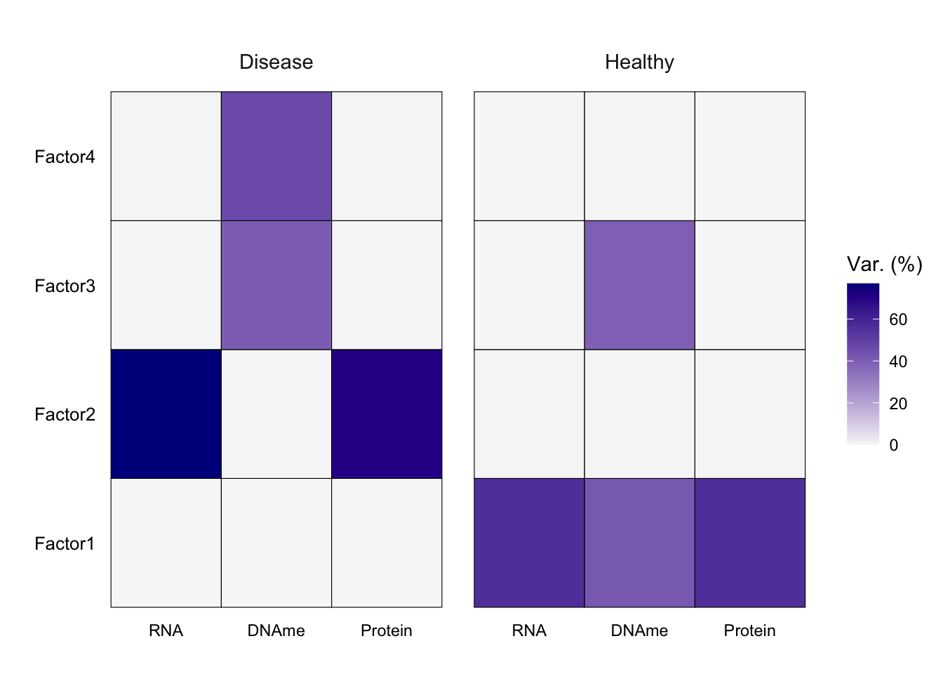
实际输出里 r2_total 显示每个组学在各组被解释的总方差(比如 RNA 在 Disease 组约 77%、Healthy 组约 56%),r2_per_factor 则给出每个因子对每个视图的方差贡献。你会发现 Factor1 主导了 Healthy 组所有视图的方差,而 Factor2 主导了 Disease 组的 RNA 和 Protein——这正是下方热图要讲的核心。需要提醒的是:不同因子解释的方差量级差异很大,个别因子(如这里的 Factor2/3/4)贡献较小,不代表它们无生物学意义,只是方差占比低。

用热图看更直观:

1
plot_variance_explained(mofa_fit)

这张图正是 MOFA 的精髓所在(颜色越深代表该因子解释的方差比例越高):

  • Factor1(最下面一行)在 Healthy 组对 RNA、DNAme、Protein 都有较强信号(深紫),而在 Disease 组几乎不解释方差——这是一个在 Healthy 组占主导的因子
  • Factor2 只在 Disease 组对 RNA 和 Protein 有强信号(深蓝),在 Healthy 组几乎为 0——这是组特异因子(只在疾病组活跃),可能捕捉疾病相关的跨组学变异;
  • Factor3 / Factor4 主要解释 DNAme 的方差(两个组的 DNAme 列都有信号),是视图特异因子,代表甲基化特有的变异维度。

注意:每个因子的"活性"是组特异视图特异的——一个因子可能只在一组、且只在部分组学里活跃。能同时区分"跨组学共享"“组特异"“视图特异"信号,正是 MOFA+ 相对普通 PCA 的突出能力。这也提醒我们:解读因子时必须结合组与视图两个维度。

4. 解释因子:载荷的可视化

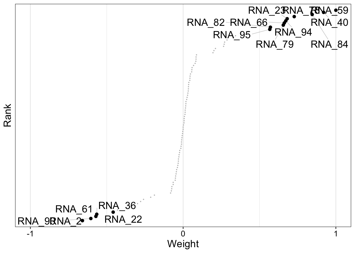
要回答"某个因子在生物学上代表什么”,需要看它在哪些特征上有大载荷。用 plot_weights() 展示因子在某个视图中的 Top 特征:

1
2
# Factor1 在 RNA 视图中的 Top 15 载荷
plot_weights(mofa_fit, view = "RNA", factor = 1, nfeatures = 15)

条形图按载荷大小排列,正负载荷分别表示该特征与因子正/负相关。

5. 因子与样本分组 / 协变量的关系

MOFA 找到的因子常与生物学状态相关。用 plot_factor() 按协变量着色,查看因子值是否区分组别:

1
2
# 按疾病状态着色,看 Factor1 是否区分
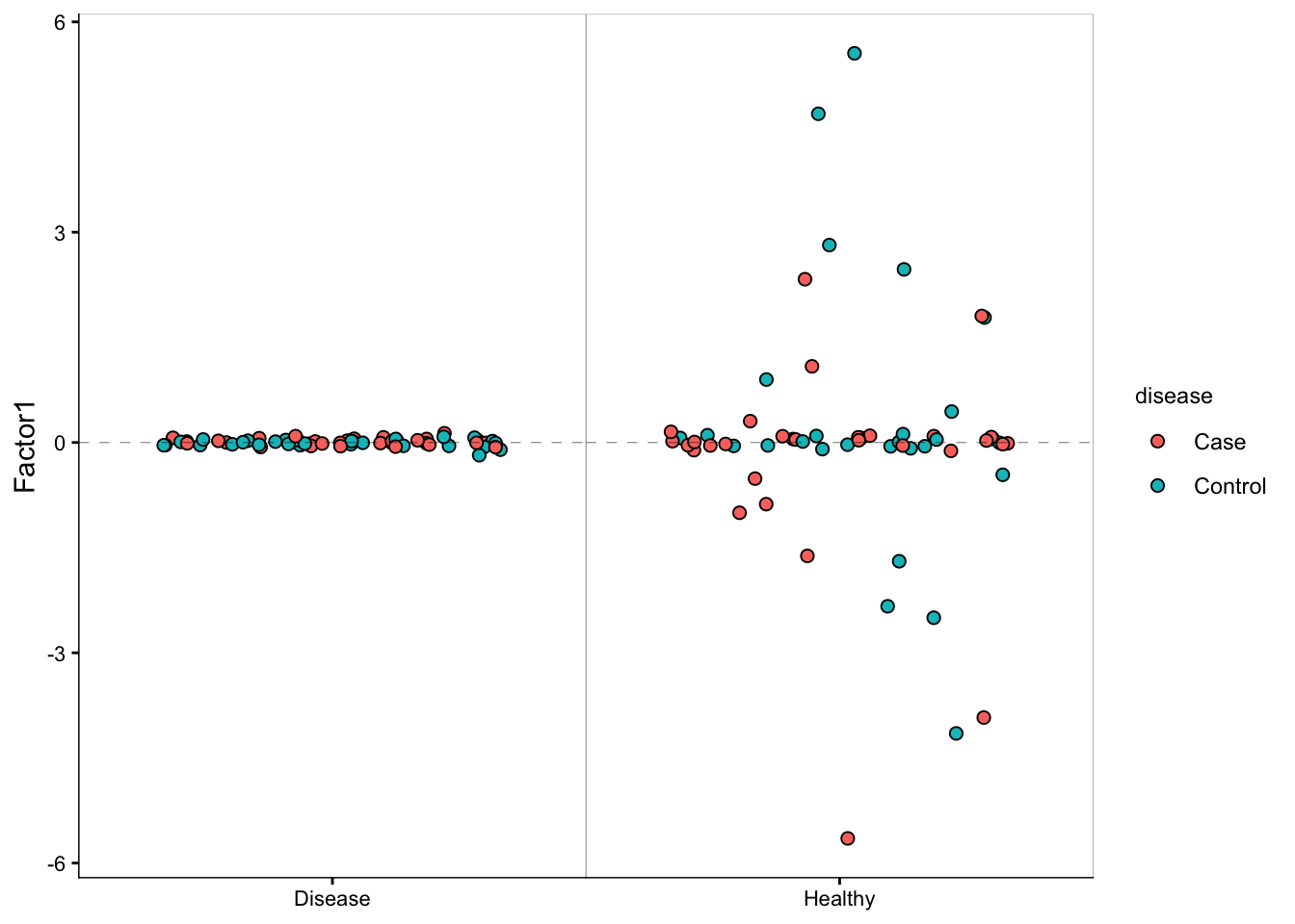
plot_factor(mofa_fit, factors = 1, color_by = "disease")

可以看到 Factor1 在 Disease 组聚集在 0 附近,而 Healthy 组散布范围大——说明 Factor1 捕捉到两组间的结构差异。这是后续关联分析的基础。

6. 因子与协变量的定量关联

更严谨的做法是计算因子得分与协变量的回归。由于多组结构下 get_factors() 按组返回、列名带组前缀,这里演示合并两组后,用线性回归检验因子与疾病状态的关联(教学示例):

 1
 2
 3
 4
 5
 6
 7
 8
 9
10
11
12
13
14
15
16
17
18
19
20
21
22
23
24
25
26
27
28
29
30
31
32
33
34
# 多组结构下 get_factors() 返回的列名带 "组名." 前缀(如 "Healthy.Factor1"),
# 这里用一个辅助函数去掉前缀,再把 sample 作为列名拼进数据框
get_clean_factors <- function(g) {
  m <- get_factors(mofa_fit, groups = g) |> as.data.frame()
  colnames(m) <- sub(paste0("^", g, "."), "", colnames(m))
  m$sample <- rownames(m)
  m$group  <- g
  m
}
factors_df <- bind_rows(lapply(groups_names(mofa_fit), get_clean_factors))

# 关联元数据中的协变量 disease(case / control)
factors_df <- factors_df |>
  left_join(samples_metadata(mofa_fit)[, c("sample", "disease")], by = "sample")

# 用线性回归检验 Factor1 是否与疾病状态相关
fit_lm <- lm(Factor1 ~ disease, data = factors_df)
summary(fit_lm)
## 
## Call:
## lm(formula = Factor1 ~ disease, data = factors_df)
## 
## Residuals:
##     Min      1Q  Median      3Q     Max 
## -5.5247 -0.1452  0.0085  0.1507  5.4287 
## 
## Coefficients:
##                Estimate Std. Error t value Pr(>|t|)
## (Intercept)     -0.1232     0.1519  -0.811    0.419
## diseaseControl   0.2463     0.2149   1.146    0.254
## 
## Residual standard error: 1.177 on 118 degrees of freedom
## Multiple R-squared:  0.01102,	Adjusted R-squared:  0.002634 
## F-statistic: 1.314 on 1 and 118 DF,  p-value: 0.2539

p 值显著,说明该因子与疾病状态相关,可作为下游解读的线索。

进阶:模型诊断与选择

1. 选择合适的因子数

MOFA 靠 ARD 机制自动决定"有效因子”——初始给足因子数(如 15),训练后不解释方差的因子会自动被剔除。因此初始 num_factors 设大一些是安全的。也可比较不同因子数下的 ELBO:

1
2
3
# 训练后查看 ELBO(越大越好)
plot_elbo <- get_elbo(mofa_fit)
plot_elbo()

实际项目中的经验做法:设置 num_factors = 15,用 convergence_mode = "slow" 跑一次,观察保留的因子数;若太多或太少再调整。

2. 检查是否有"技术性因子"

训练后 MOFA2 会给出 QC 警告,例如"某因子与总表达特征数强相关"。出现这类警告时,该因子可能捕捉的是文库大小 / 批次效应而非生物学信号,应结合载荷与协变量关联判断是否剔除。

3. 缺失值与其它似然

MOFA 天然支持缺失值(概率模型可从观测数据推断),这是它相比普通 PCA 的又一优势。若组学是计数数据(如 RNA 计数),把对应的 likelihoods 设为 "poisson";二值数据设为 "bernoulli"

MOFA 的优缺点

优点

  1. 真正的多组学整合:共享潜因子把不同组学放在同一坐标系,自动识别跨组学信号。
  2. 无监督、可解释:不需要标签即可降维,因子可通过载荷和协变量关联解释。
  3. 视图与组双重稀疏:ARD 先验自动决定"哪些因子在哪些视图/组中活跃",避免人为设定。
  4. 支持多组结构:MOFA+ 能区分共享因子与组特异因子,适合多队列、多批次分析。
  5. 容忍缺失值:概率模型可处理部分组学缺失的样本。
  6. 下游分析友好:因子得分可直接用于 MANOVA、回归、聚类与可视化。

局限性

  1. 依赖 Python 后端:需要额外安装 mofapy2,环境配置是主要门槛。
  2. 计算开销:样本和特征很多时,变分推断耗时较长(可用 stochastic 随机变分近似加速)。
  3. 对预处理敏感:中心化、缩放、归一化的选择会影响因子;原始 count 数据需先正确转换。
  4. 因子解释需要背景知识:MOFA 输出的是统计因子,其生物学语义需结合载荷与协变量关联人工解读。
  5. 高斯假设为主:默认 gaussian 似然;非正态组学需显式指定其它似然。

注意事项

  • 样本对齐:所有视图必须共享相同样本且列顺序一致,这是最常踩的坑。
  • 预处理是前提:先做质量控制、批次校正(如 removeBatchEffect)与归一化,再喂给 MOFA,否则因子会被技术噪音主导。
  • 设置随机种子train_opts$seed 保证可复现,MOFA 训练是随机初始化的。
  • 区分生物与技术因子:结合协变量关联和 QC 警告,识别并剔除技术性因子。
  • 特征命名:给特征加视图前缀(如 RNA_DNAme_),否则不同视图的特征同名会混淆。

从示例数据迁移到真实数据

data_list 换成你自己的多组学矩阵即可,格式要求是:

 1
 2
 3
 4
 5
 6
 7
 8
 9
10
data_list <- list(
  RNA     = rna_matrix,       # 特征 × 样本
  DNAme   = meth_matrix,      # 特征 × 样本
  Protein = protein_matrix    # 特征 × 样本
)
# 必须确保所有矩阵列名(样本)一致且顺序相同
stopifnot(identical(colnames(data_list$RNA), colnames(data_list$DNAme)))

# 可选:提供样本元数据(含 group 列)
samples_meta <- data.frame(sample = colnames(data_list$RNA), group = ..., ...)

后续 create_mofaprepare_mofarun_mofa 完全一样。若数据是稀疏矩阵或过大,可用 create_mofa(..., extract_metadata = FALSE) 等方式控制内存。

参考文献与扩展

  • Argelaguet, R., et al. (2018). Multi-Omics Factor Analysis—a framework for unsupervised integration of multi-omics data sets. Molecular Systems Biology, 14(6), e8124.
  • Argelaguet, R., et al. (2020). MOFA+: a statistical framework for comprehensive integration of multi-modal single-cell data. Genome Biology, 21, 111.
  • MOFA2 官方文档与教程:https://biofam.github.io/MOFA2/
  • 相关扩展:MOFA2run_mofa 底层是 mofapy2MEFISTO(时空因子分析)可通过 mefisto_options 配置。
  • 集成到单细胞分析:MOFA+ 可与 Seurat / Scanpy 的降维结果关联,用于多模态单细胞整合。

小结

多组学因子分析(MOFA)用概率矩阵分解 + ARD 稀疏先验,把多种组学整合进同一组共享潜因子,既能降维,又能揭示跨组学共享信号与组/视图特异性信号。本文用 MOFA2 包 + 合成三组学数据走通了完整流程:准备数据 → 创建对象 → 配置参数 → 训练 → 解读方差解释与载荷 → 因子与协变量关联 → 模型诊断。掌握这套流程,你就能在自己的多组学数据上挖掘跨组学的结构信号。

Email: pengchen2001@zju.edu.cn
Built with Hugo
Theme Stack designed by Jimmy